
Modelling is an act of reality conceptualization. It is thus directly related to a simplification process where one applies a theory with limited validity to a physical realization. A good model should be the simplest and most representative idealization of the system under study. A trade-off is then at play between implementation complexity and experimental correlation, biased by the ability to measure the relevant information and identify associated model values. This gets us to the popular statement attributed to George Box: “All models are wrong, but some are useful”.
That said, to be useful the model should be right enough! The line must indeed be drawn between model limitations that should be assessed (validation process), and implementation/interpretation mistakes that should be avoided (verification process). We have sometimes seen in the industry this line getting blurred for various reasons. The lack of exploitable experimental values is indeed a common challenge for modelling and simulations. Input values are required to run a model, restricted by the purchased software implementation, and one will sometimes have to guess a value or globally ignore a phenomenon to produce a result.
Our take for such challenge is to get back to the physics at play in the system and assess model sensitivity to the unmastered phenomenon at stake. To do so it is interesting to start by considering parameters associated with the effects induced by the phenomenon rather than directly using a detailed model. We develop correlation methods such as the Minimum Dynamic Residue Expansion (MDRE) method [1] that is effective at challenging models with a critical eye on test data, and our tools provide enough flexibility to implement new model variations related to the behavior that would be induced by the phenomenon. Should the model be sensitive, the next steps will be required, but at least validation limitations are assessed, and the model will be verified in the process.
To illustrate what this discussion means in structural dynamics, we will use a disc brake system. We have been studying brake squeal for many years, and the models are usually quite complex, involving around ten components in interaction. Squeal noise is emitted when the system is unstable due to friction induced vibrations that couples in-plane and out-of-plane displacements at the braking interface, here between the pads and the disc. Squeal is a non-linear phenomenon, linked to unstable linear modes that are usually characterized in simulation [2].
Brake system and pressure actuation modelling
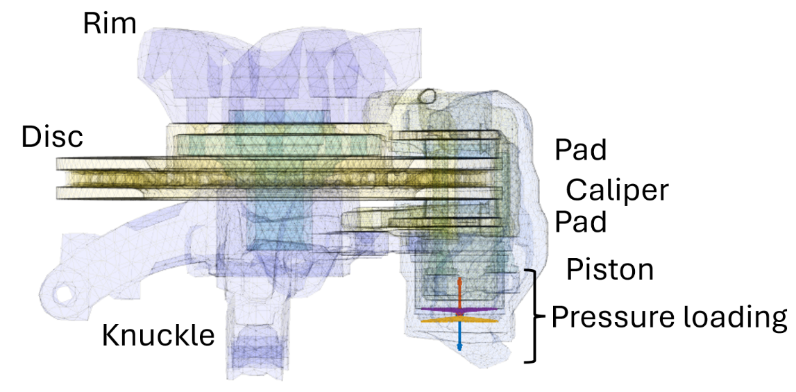
Automotive disc brakes mostly use hydraulic actuation. The caliper is fitted with piston(s) that will push the braking pads onto the disc. Floating caliper systems will use piston(s) on a single side and a sliding mechanism will let the caliper move to apply pressure on the second side. Coming from a mechanical perspective, the brake fluid and flanges are not modelled, and pressure as distributed loads are directly applied in opposite directions to the piston butt and caliper chamber as shown in the figure.
Applying pressure and disc rotation lead to steady sliding conditions, a style of preload to be used for modal computation representative of the brake system in operation. Considering a system meshed in a braking ready position, the preload is mostly limited to the resolution of components contact conditions. These conditions lead to effective contact surfaces, characterized by the resolved pressure fields as shown below.
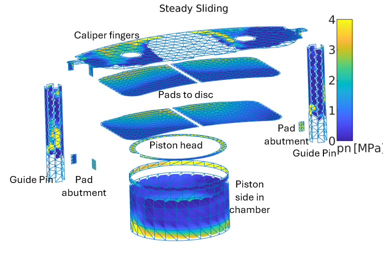
Many contacts exist, between the pads and disc, piston, caliper, and of course between the piston and caliper chamber. Model linearization for modal computation thus recovers coupling stiffness in the loaded areas only, no coupling occurs in areas with no pressure even if they were declared in the model contact surfaces. The coupling stiffnesses may depend on pressure levels depending on the contact law [3].
Regarding the hydraulic actuator, modelling simplifications must also be assessed with care for linearization. In reality a pressurized fluid is present, so that a bulk stiffness should be represented, but as only a pressure load has been modeled no stiffness will be derived during linearization by the solver! Not adding stiffness is thus wrong and as it will significantly alter the stiffness stack between the disc and caliper, results will be useless.
Adding a bulk stiffness to the system is however not always easy, considering the fact that its effect may be coupled to friction effects between the piston and caliper. Indeed, as a contact interaction is present between the piston side and caliper in the model, considering a friction coefficient in the interaction will lead to an adhesive stiffness in the linearized model.
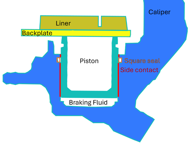
Most models will consider adhesion stiffness based on the contact stiffness tending to provide a high value even for low friction coefficients. The fluid bulk stiffness may thus get overridden by piston side adhesion bias in the model, making it apparently unsensitive… Is it equivalent? Certainly not! What models should be implemented is another question. Heuristics leads one to think that due to the fluid pressure, piston sides should be rather free to slide with a weak adherence, while the bulk stiffness should be high.
Assessing modelling sensitivity to pressure application models
Experimental correlation would allow progressing towards identifying the best values [4]. In this post we will illustrate the complex eigenvalues sensitivity to brake fluid bulk stiffness and piston side adherence. One thus considers the illustrated brake model linearized at the given steady sliding preload. Two parameters are considered
- HouPiKt represents a modulation of the piston to caliper side adherence defined as an adhesive stiffness. Values are varied between 10-6 (~zero stiffness) to 10 (~fully sticked).
- BkPiStiff represents the fluid bulk stiffness, here implemented using a stiffness associated to the pressure load command. Movements opposing pressure application thus get penalized. A nominal stiffness of 106 N/mm is considered, a coefficient between 10-6 (no stiffness) and 106 (~imposed displacement constraint) is varied. Despite the fact that a physical value has not been estimated a transition between nothing and very stiff will help identifying sensitive values and provide clues for experimental identification in case of need.
A factorial (or full grid) design of experiment considering a logarithmic evolution discretized into 75 values for each parameter is considered, leading to 5625 design points. A parametrized reduced order multi-model is generated based on three full points [5], so that such study can be generated in a couple hours and under 10GB for 100 modes of a multi-million DOF system, keeping all shapes.
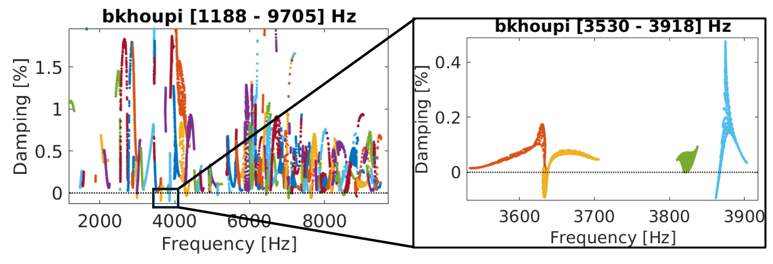
The results are given in the figure below in the form of a root locus, or stability diagram, displaying all system modes frequency and damping for each sampled configuration. Modes with negative damping are unstable and thus of particular interest. A zoom-in on 3.6-3.9 kHz is given at the location of one of the brake unstable modes. Looking at the root locus it is not unstable for every configuration, and several unstable frequencies seem to exist.
To understand the variations between these shapes and their parametric existence, a PoleCluster study is performed. This process implemented in our SDT-ZParam module performs a classification of modeshapes using the subspace angle metric and a clustering algorithm [5]. It resorts that two different unstable modes exist, with different bracket deformations
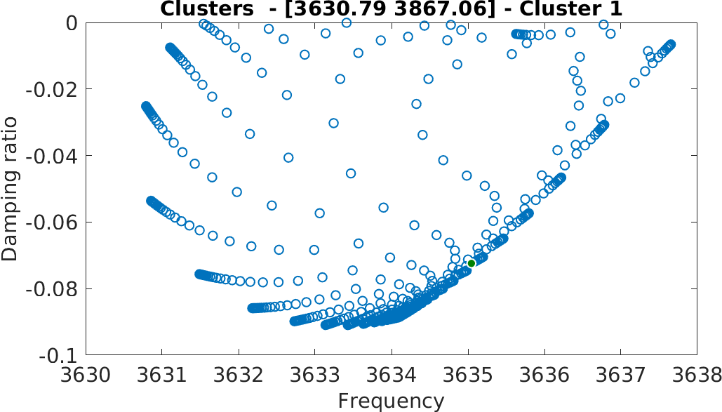
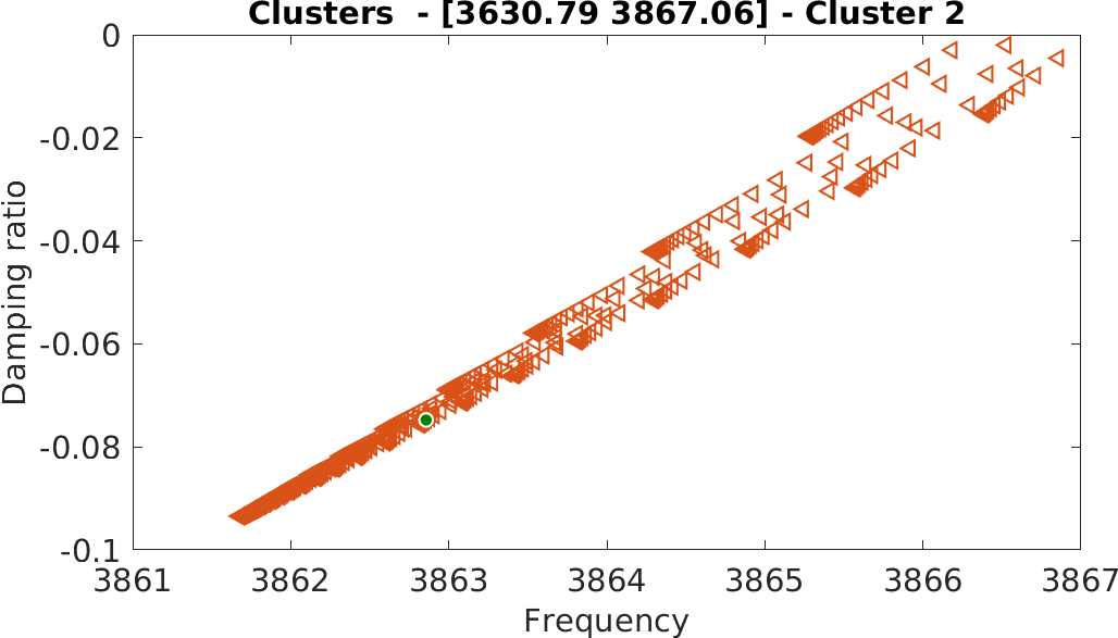
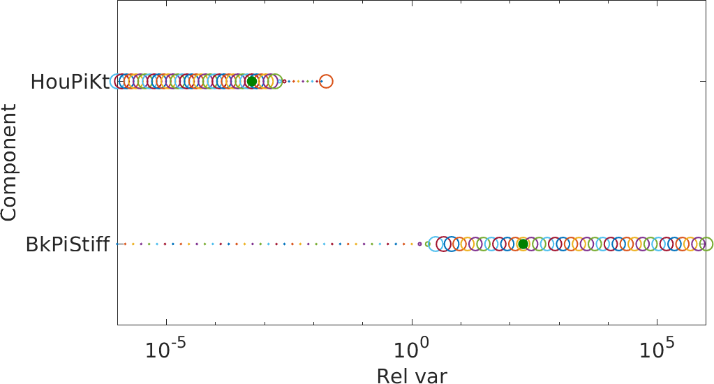
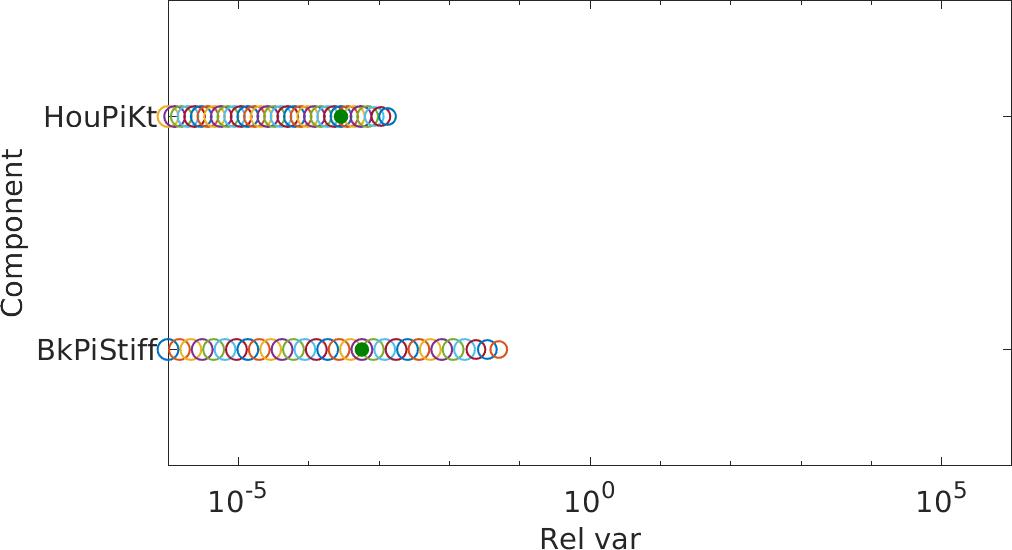
Parameter distribution for both clusters provide insightful observations. First, both clusters exist only for small values of piston side adhesive stiffness. With the physical assessment that adherence should be low, adding a small friction coefficient for steady sliding simulation and not altering the associated adhesive stiffness in the linearization process would lead to missing an unstable mode.
Second, the unstable mode shape and frequency depends on the brake fluid bulk stiffness. While this value may also depend on the actually applied pressure, experimental correlation would give more clues about the effective bulk stiffness by comparing the frequencies and shapes.
Conclusion
The simplifications implied by a modelling strategy must be verified for each simulation procedure. The derivations, linearizations, reductions performed come each with their additional set of assumptions and commercial software implementations that may not be coherent with the user’s objectives.
It can be easy to miss specific aspects, as presented in this post dealing with brake squeal and pressure actuator modelling, that often requires corrections in the models we receive. This case is not trivial as with the steady sliding preload, component coupling is never zero. Visually bad results such as free flying components thus do not happen. Omitting brake fluid bulk stiffness may well be compensated by keeping adhesive stiffness at other interfaces. The simulation outcome will however be different enough to significantly change the analysis results.
Having the right tools to perform verification and validation is then critical. At SDTools, we aim at providing such solutions to develop useful models!
References
![]()
[1] Expansion in structural dynamics: a perspective gained from success and errors in test/FEM twin building
![]()
[2] Squeal complex eigenvalue analysis, advanced damping models and error control
![]()
[3] Benchmarking Signorini and exponential contact laws for an industrial train brake squeal application.
![]()
[4] MDRE: An efficient expansion tool to perform model updating from squeal measurements
![]()
[5] Efficient Large Multi-Parametric Squeal Simulation And Analysis Using Advanced Model Reduction Tools