
🎯 In structural dynamics as in any other field, prototyping is a key project validation step. To reduce as much as possible the costly experimental phase, simulation is employed to refine design and ensure compliance with objectives as much as possible.
✅ Validation requires an experimental correlation with the simulation. Measurements have to be realized through sensors. In mechanics, it is typical to measure local features as
- Displacement (eddy current probes)
- Velocity (laser doppler vibrometer)
- Acceleration (piezo accelerometers)
- Force (load cell)
- Strain (strain gauges)
This post topic is about using sensors in a model, and how this can be used to optimize a test campaign. In SDT, that provides many tools associated with experimental correlation, sensors are natively handled through a Case entry of type SensDof, where every imaginable type can be defined. Our definition approach is based on a tabulated list documented in https://www.sdtools.com/helpcur/base/scell.html#scell.
Processing sensor input leads to the generation of a sens data type https://www.sdtools.com/helpcur/base/sstruct.html#sens.tdof featuring our internal tdof table linking the sensor to its observation on the finite element model. In standard cases, it links the sensor ID to a node (test wireframe of FEM) and a direction – a triax is transformed into three distinct sensors.
Associating a sensor measure with the FEM data requires a matching procedure that we call topology correlation. Sensor positions are projected on the mesh, and the finite element shape functions are interpolated to obtain what the sensor must measure. For forces and strains the constitutive laws are involved. At low level we use the SensMatch procedure https://www.sdtools.com/helpcur/base/sensor.html#SensMatch. This is integrated and interfaced at a higher level in our DockCoTopo GUI: https://www.sdtools.com/help/base/dockCoTopo.html.
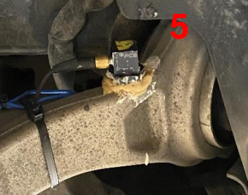
The most common solution for experimental vibration analysis is to use accelerometers, as it is usually a cost-effective solution with good working ranges in vibration applications. They can be uniaxial or triaxial and have to be fixed to the component surface at measurement location. Studs or adhesive fixation are the most two common techniques. Studs require some drilling. Gluing is a delicate phase as the “glue” material should be stiff enough to generate a strong connection for the frequency, temperature and amplitude of interest while being sufficiently easy to remove without damage to the accelerometer, several kinds of mastic, glues, or petro-wax can be used.
Adding accelerometers to a component modifies it. Each accelerometer has its own mass (also considering the connection cable), its own local measurement directions, and also provides an offset measurement from the component surface. All these aspects have to be assessed and sometimes accounted for – this will be the topic of another post, stay tuned!
In this post we will present the basics of sensor and actuator definition for a test campaign, assessing the following points:
👉 How to perform sensor positioning ?
👉 How to check sensor positioning quality ?
👉 How to perform actuator positioning ?
I – Sensor positioning
Defining sensor position is not always an easy task without prior knowledge of the system behavior. Missing some important features will require another test campaign. Simulation can help with this task by providing optimal sensor positions, and excitation points.
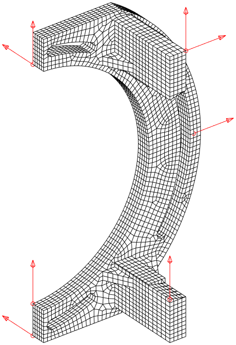
To illustrate how to optimize a test campaign regarding sensor and excitation positioning a sample bracket component that we studied in the past will be used, we call it the banana. This bracket has some very interesting features as its dimensions and voids generate many modes at frequencies close to automotive axle components. Besides it is almost symmetrical and can be used to demonstrate other correlation peculiarities. A few of the banana modes are illustrated below:
A good sensor positioning strategy aims at being able to observe all desired modes and to be able to distinguish modeshapes.
- Observing with enough magnitude should target location with high values homogeneous to measurement method, high displacement, or high strain locations depending on the case.
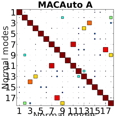
- Being able to distinguish between modes means that measured features must be different enough for each mode, this is usually checked with an auto-MAC, where out-of-diagonal terms characterize the level of distinction one can have between each shape pairs.
SDT provides for displacement based sensors a sequential placement algorithm named MSeq https://www.sdtools.com/helpcur/base/fe_sens.html#mseq. It generates a number targeted list of DOF to maximize observability and dinstiguability. The example below shows the result obtained when asking for 10 sensors to measure the first 18 modes under 6kHz.
The result with 10 sensors is not perfect as a few mode pairs still cannot be distinguished. The pair 7-11 is illustrated below. With the provided set of sensors, the handle and foot movements are well caught, but they tend to be similar for this pair. Differences appear more on the body.
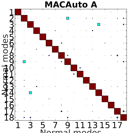
The MSeq algorithm can then be used to add sensors to the pre-existing list until we get a better result. For 18 modes an almost perfect diagonal auto-MAC is obtained with 17 sensors, displayed in the figure below. Due to the banana symmetry and high handle flexibility almost a sensor per mode is required!
A classical limitation with automated sensor placement algorithms is linked to the fact that displacement tends to be maximal at the geometry extremities. Ideally optimal position thus tends to be on edges or sharp edges, that are difficult to handle practically when the operator has to fix the sensor and/or hit the location with a hammer.
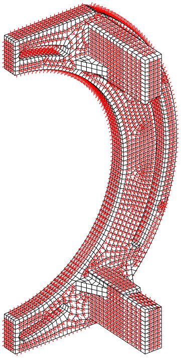
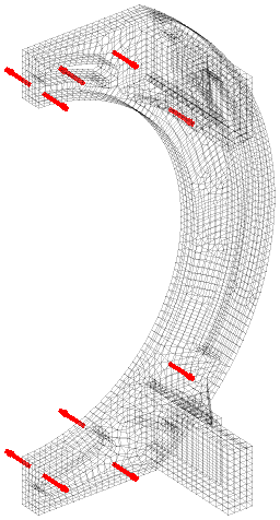
To alleviate this shortcoming, we developed the In-Acceptable functionality https://www.sdtools.com/helpcur/base/fe_sens.html#InAcceptable that automatically discards sharp edges, small facets, and invisible faces (for laser pointing). A sublist of acceptable DOF for measurement is then provided to work with MSeq and other algorithms. In our banana example, the list of acceptable locations is highlighted in red in the figure below. The MSeq algorithm is run in this subset and provides locations close to the previous ones but further from the sharp edges. The specification thus becomes more precise, giving a better chance for a better topology correlation.
II – Going further with fixed sensor modes
Adding sensors using the model can be very helpful, but what if the model was not fully predictive? For a simple component, one can get confident, as long as a single homogeneous isotropic material is used. In the case of multi-materials, contact interactions, fastenings, or non homogeneous and/or non isotropic materials (additive manufacturing, sintering…), … even a single component can become complicated.
If the model is not fully predictive the modeshapes may be different from the ones we calibrated the sensors on. In such case a useful indicator is the frequency at which you will start possibly missing shape information. It can be accessed by computing the fixed sensor modes. Reminding the fact that a sensor is transformed into an observation equation on the finite element model,
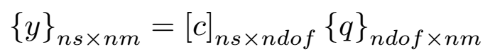
where [c] is the observation matrix, one can also use this observation as a general Multiple Point Constraint (MPC). The sensors here become control points. By fixing them all and computing the associated modes, one gets the movements that are not constrained by the sensor equations, thus not observable.
For our flexible banana, with the previously defined 17 sensors, the first two fixed sensor modes are displayed in the figure below. It is in fact very low and the attentive reader will note that it is even under the first flexible mode, which means that our set of sensors do not fully constrain rigid body modes.
The first fixed sensor mode shows an horizontal translation of the lower column, coherent with the fact that no horizontal translation is measured on the lower side. Adding a sensor there improves the behavior, and one can iterate this way until getting to a high enough minimal frequency

This process can be repeated as long as needed. It clearly highlights the fact that having enough sensors to distinguish between a given set of modes is different from ensuring that every movement under a given frequency threshold is captured!
Using triax sensors may help generating more sensors at less locations. For our example using the original 10 localization points with triax directly generates 30 sensors and gets the first fixed sensor mode close to 2kHz.
III – Making sure we excite the modes
The second side of being able to observe a mode resides in the capability to generate a modal response in the direction of the modes of interest. Excitation is commonly performed with an impact hammer or a shaker for experimental modal analysis. One can then try to optimize the excitation point by finding a location where the target modes are observable. Indeed, observability and controlability are equivalent for a linear response.
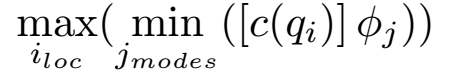
For a given set of control DOF, one will thus look for the DOF whose minimal controlability over all target modes is maximal:
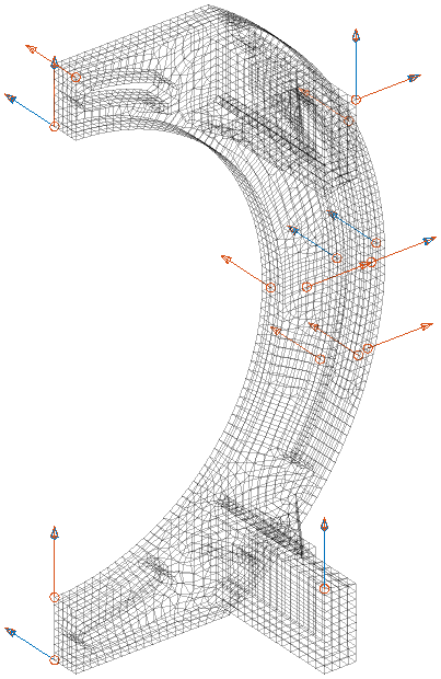
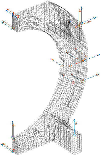
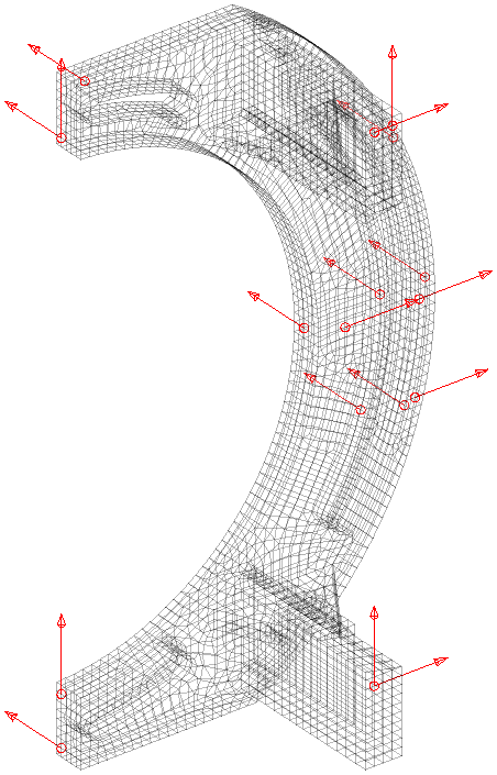
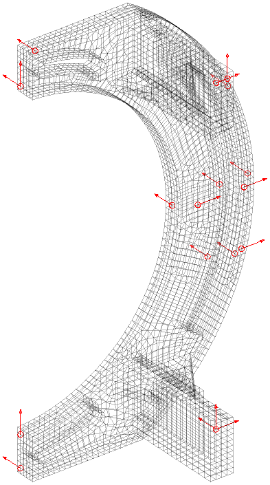
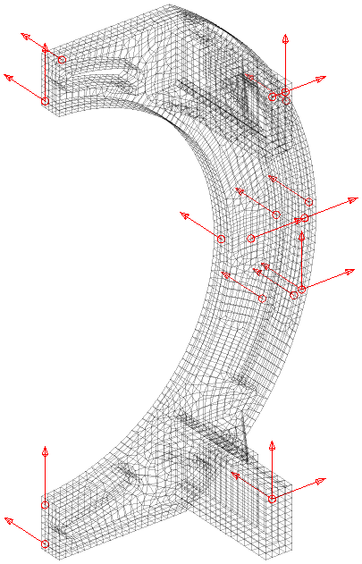
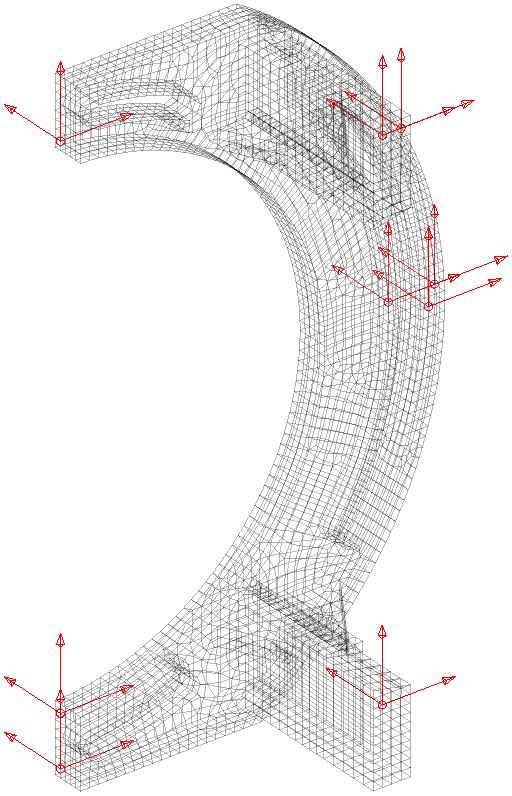
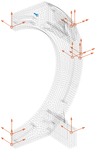
Orientation of the excitation has to be accounted for, and for a hammer, one will look for directions normal to the surface. SDT provides a tool to recover normal surface displacement with our command NormalVel https://www.sdtools.com/helpcur/base/fe_sens.html. The observation matrix to use will then be a surface normal displacement direction restricted to acceptable locations. For our banana, the first ten locations providing maximum controlability potential is given below.
A final check can then be performed by simulating the transfers using the selected inputs and outputs. Our sample setup uses the 10 triax previously selected and an impact point among the best ones.
Using the normal modes for the transfer with a uniform modal damping of 0.5%, the transfers can be quickly synthesized using function nor2xf https://www.sdtools.com/help/base/nor2res.html. A post-treatment to display the sum of all imaginary parts (SUMI) or the MMIF indicator associated with pole markers allows ensuring that every mode is theoretically excited and visible.
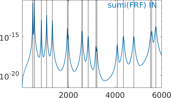
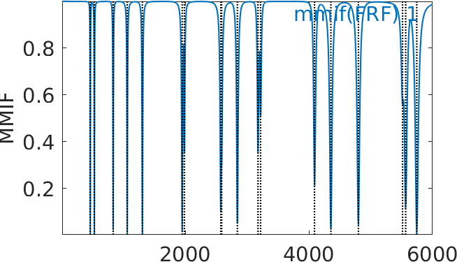
On this response you see that some modes are very close in frequency and are in fact doubles modes associated to the banana columns bending. Further optimization could be done to ensure a good ability to observe these modes separately. Multiple excitation points would be necessary in practice and SDT also provides a MMIF optimization function to provide optimal multiple localization targeting specific modes.
Many other features and effects associated with sensors can be discussed above the concepts presented here, and we will soon get back to this topic in the future.