PDF Index
|
Contents
Functions
PDF Index |
Three kinds of manipulations are possible using the feplot GUI
feplot figures are used to view FE models and hold all the data needed to run simulations. Data in the model can be viewed in the property figure (see section 4.1.3). Data in the figure can be accessed from the command line through pointers as detailed in section 4.1.2. The feplot help gives architecture information, while fecomlists available commands. Most demonstrations linked to finite element modeling (see section 1.2 for a list) give examples of how to use feplot and fecom.
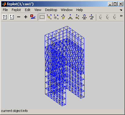
Figure 4.1: Main feplot figure.
The first step of most analyzes is to display a model in the main feplot figure. Examples of possible commands are (see fecom load for more details)
As an example, you can load the data from the gartfe demo, get cf a SDT handle for a feplot figure, set the model for this figure and get the standard 3D view of the structure
 model=demosdt('demogartfe')
 cf=feplot;       % open FEPLOT and define a pointer CF to the figure
 cf.model=model;
The main capabilities the feplot figure are accessible using the figure toolbar, the keyboard shortcuts, the right mouse button (to open context menus) and the menus.
List of icons used in GUIs
 | Model properties used to edit the properties of your model. |
 | Start/stop animation |
 | Previous Channel/Deformation |
 | Next Channel/Deformation |
 | iimouse zoom |
 | Orbit. Remaining icons are part of MATLAB cameratoolbar functionality. |
 | Snapshot. See iicom ImWrite. |
At this level note how you can zoom by selecting a region of interest with your mouse (double click or press the i key to zoom back). You can make the axis active by clicking on it and then use any of the u, U, v, V, w, W, 3, 2 keys to rotate the plot (press the ? key for a list of iimousekey shortcuts).
The contextmenu associated with your plot may be opened using the right mouse button and select Cursor. See how the cursor allows you to know node numbers and positions. Use the left mouse button to get more info on the current node (when you have more than one object, the n key is used to go to the next object). Use the right button to exit the cursor mode.
Notice the other things you can do with the ContextMenu (associated with the figure, the axes and objects). A few important functionalities and the associated commands are
The figure Feplot menu gives you access to the following commands (accessible by fecom)
cf1=feplot returns a pointer to the current feplot figure. The handle is used to provide simplified calling formats for data initialization and text information on the current configuration. You can create more than one feplot figure with cf=feplot(FigHandle). If many feplot figures are open, one can define the target giving an feplot figure handle cf as a first argument to fecom commands.
The model is stored in a graphical object. cf.model is a method that calls fecom InitModel. cf1.mdl is a method that returns a pointer to the model. Modifications to the pointer are reflected to the data stored in the figure. However mo1=cf.mdl;mo1=model makes a copy of the variable model into a new variable mo1.
cf.Stack gives access to the model stack as would cf.mdl.Stack but allows text based access. Thus cf.Stack{'EigOpt'} searches for a name with that entry and returns an empty matrix if it does not exist. If the entry may not exist a type must be given, for example cf.Stack{'info','EigOpt'}=[5 10 1].
cf.CStack gives access to the case stack as would calls of the form
Case=fe_case(cf.mdl,'getcase');stack_get(Case,'FixDof','base') but it allows more convenient string based selection of the entries.
cf.Stack and cf.CStack allow regular expressions text based access. First character of such a text is then #. One can for example access to all of the stack entries beginning by the string test with cf.Stack{'#test.*'}. Regular expressions used by SDT are standard regular expressions of Matlab. For example . replaces any character, * indicates 0 to any number repetitions of previous character...
Finite element models are described by a data structures with the following main fields (for a full list of possible fields see section 7.6)
| .Node | nodes |
| .Elt | elements |
| .pl | material properties |
| .il | element properties |
| .Stack | stack of entries containing additional information cases (boundary conditions, loads, etc.), material names, etc. |
The model content can be viewed using the feplot property figure. This figure is opened using the icon, or fecom('ProInit').
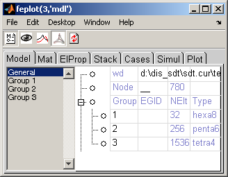
Figure 4.2: Model property interface.
This figure has the following tabs
 mode, associated elements in selection are shown. See section 4.2.1.
The figure icons have the following uses
| | Model properties used to edit the properties of your model. |
| Active display of current group, material, element property, stack or case entry. Activate with fecom('ProViewOn'); |
 | Open the iiplot GUI. |
 | Open/close feplot figure |
 | Refresh the display, when the model has been modified from script. |
Hand declaration of a model can only be done for small models and later sections address more realistic problems. This example mostly illustrates the form of the model data structure.
Figure 4.3: FE model.
The geometry is declared in the model.Node matrix (see section 7.1 and section 7.1.2). In this case, one defines 6 nodes for the truss and an arbitrary reference node to distinguish principal bending axes (see beam1)
 %     NodeID  unused   x y z
 model.Node=[ 1      0 0 0    0 1 0; ...
              2      0 0 0    0 0 0; ...
              3      0 0 0    1 1 0; ...
              4      0 0 0    1 0 0; ...
              5      0 0 0    2 0 0; ...
              6      0 0 0    2 1 0; ...
              7      0 0 0    1 1 1]; % reference node
The model description matrix (see section 7.1) describes 4 longerons, 2 diagonals and 2 battens. These can be declared using three groups of beam1 elements
 model.Elt=[ ...
  % declaration of element group for longerons
  Inf     abs('beam1') ; ...
  %node1  node2   MatID ProID nodeR, zeros to fill the matrix
    1       3      1    1     7       0 ; ...
    3       6      1    1     7       0 ; ...
    2       4      1    1     7       0 ; ...
    4       5      1    1     7       0 ; ...
  % declaration of element group for diagonals
  Inf     abs('beam1') ; ...
    2       3      1    2     7       0 ; ...
    4       6      1    2     7       0 ; ...
  % declaration of element group for battens
  Inf     abs('beam1') ; ...
    3       4      1    3     7       0 ; ...
    5       6      1    3     7       0 ];
You may view the declared geometry
 cf=feplot; cf.model=model;       % create feplot axes
 fecom(';view2;textnode;triax;'); % manipulate axes
The demo_fe script illustrates uses of this model.
Declaration by hand is clearly not the best way to proceed in general.femesh provides a number of commands for finite element model creation. The first input argument should be a string containing a single femesh command or a string of chained commands starting by a ; (parsed by commode which also provides a femesh command mode).
To understand the examples, you should remember that femesh uses the following standard global variables
| FEnode | main set of nodes |
| FEn0 | selected set of nodes |
| FEn1 | alternate set of nodes |
| FEelt | main finite element model description matrix |
| FEel0 | selected finite element model description matrix |
| FEel1 | alternate finite element model description matrix |
In the example of the previous section (see also the d_truss demo), you could use femesh as follows: initialize, declare the 4 nodes of a single bay by hand, declare the beams of this bay using the objectbeamline command
 FEel0=[]; FEelt=[];
 FEnode=[1 0 0 0  0 0 0;2 0 0 0    0 1 0; ...
         3 0 0 0  1 0 0;4 0 0 0    1 1 0]; ...
 femesh('objectbeamline 1 3 0 2 4 0 3 4 0 1 4');
The model of the first bay in is now selected (stored in FEel0). You can now put it in the main model, translate the selection by 1 in the x direction and add the new selection to the main model
 femesh(';addsel;transsel 1 0 0;addsel;info');
 model=femesh('model');  % export FEnode and FEelt geometry in model
 cf=feplot; cf.model=model;
 fecom(';view2;textnode;triax;');
You could also build more complex examples. For example, one could remove the second bay, make the diagonals a second group of bar1 elements, repeat the cell 10 times, rotate the planar truss thus obtained twice to create a 3-D triangular section truss and show the result (see d_truss)
 femesh('reset');
 femesh('test2bay');
 femesh('removeelt group2');
 femesh('divide group 1 InNode 1 4');
 femesh('set group1 name bar1');
 femesh(';selgroup2 1;repeatsel 10 1 0 0;addsel');
 femesh(';rotatesel 1 60 1 0 0;addsel;');
 femesh(';selgroup3:4;rotatesel 2 -60 1 0 0;addsel;');
 femesh(';selgroup3:8');
 model=femesh('model0');  % export FEnode and FEel0 in model
 cf=feplot; cf.model=model;
 fecom(';triaxon;view3;view y+180;view s-10');
femesh allows many other manipulations (translation, rotation, symmetry, extrusion, generation by revolution, refinement by division of elements, selection of groups, nodes, elements, edges, etc.) which are detailed in the Reference section.
Other more complex examples are treated in the following demonstration scripts d_plate, beambar, d_ubeam, gartfe.
This section describes functionality accessible with the Edit list item in the Model tab. To force display use fecom('CurtabModel','Edit').
Below are sample commands to run the functionality from the command line.
model=demosdt('demoubeam');cf=feplot;
fecom('CurtabModel','Edit')
fecom(cf,'addnode')
fecom(cf,'addnodecg')
fecom(cf,'addnodeOnEdge')
fecom(cf,'RemoveWithNode')
fecom(cf,'RemoveGroup')
fecom(cf,'addElt tria3')

fe_case(cf.mdl,'rbe3','RBE3',[1 97 123456 1 123 98 1 123 99]);
fe_case(cf.mdl,'rbe3 -append','RBE3',[1 100 123456 1 123 101 1 123 102]);
fecom addRbe3
While this is not the toolbox focus, SDT supports some free meshing capabilities.
fe_gmsh is an interface to the open source 3D mesher GMSH. Calls to this external program can be used to generate meshes by direct calls from MATLAB. Examples are given in the function reference.
fe_tetgen is an interface to the open source 3D tetrahedral mesh generator. See help fe_tetgen for commands.
fe_fmesh contains a 2D quad mesher which meshes a coarse mesh containing triangles or quads into quads of a target size. All nodes existing in the rough mesh are preserved.
% build rough mesh
model=feutil('Objectquad 1 1',[0 0 0;2 0 0; 2 3 0; 0 3 0],1,1);
model=feutil('Objectquad 1 1',model,[2 0 0;8 0 0; 8 1 0; 2 1 0],1,1);
% start the mesher with a reference distance of .1
model=fe_fmesh('qmesh .1',model.Node,model.Elt);
feplot(model);
Other resources in the MATLAB environment are initmesh from the PDE toolbox and the Mesh2D package.
The base SDT supports reading/writing of test related Universal files. All other interfaces are packaged in the FEMLink extension. FEMLink is installed within the base SDT but can only be accessed by licensed users.
You can get a list of currently supported interfaces trough the
comgui('FileExportInfo'). You will find an up to date list of interfaces with other FEM codes at www.sdtools.com/tofromfem.html). Import of model matrices in discussed in section 4.1.9.
These interfaces evolve with user needs. Please don't hesitate to ask for a patch even during an SDT evaluation by sending a test case to info@sdtools.com.
Interfaces available when this manual was revised were
| ans2sdt | reads ANSYS binary files, reads and writes .cdb input (see FEMLink) |
| abaqus | reads ABAQUS binary output .fil files, reads and writes input and matrix files (.inp,.mtx) (see FEMLink) |
| nasread | reads the MSC/NASTRAN [26] .f06 output file (matrices, tables, real modes, displacements, applied loads, grid point stresses), input bulk file (nodes, elements, properties). FEMLink provides extensions of the basic nasread, output2 to model format conversion including element matrix reading, output4 file reading, advanced bulk reading capabilities). |
| naswrite | writes formatted input to the bulk data deck of MSC/NASTRAN (part of SDT), FEMLink adds support for case writing. |
| nopo | This OpenFEM function reads MODULEF models in binary format. |
| perm2sdt | reads PERMAS ASCII files (this function is part of FEMLink) |
| samcef | reads SAMCEF text input and binary output .u18, .u11 , .u12 files (see FEMLink) |
| ufread | reads results in the Universal File format (in particular, types: 55 analysis data at nodes, 58 data at DOF, 15 grid point, 82 trace line). Reading of additional FEM related file types is supported by FEMLink through the uf_link function. |
| ufwrite | writes results in the Universal File format. SDT supports writing of test related datasets. FEMLink supports FEM model writing. |
FEMLink handles importing element matrices for NASTRAN (nasread BuildUp), ANSYS (ans2sdt BuildUp), SAMCEF (samcef read) and ABAQUS (abaqus read).
Reading of full matrices is supported for NASTRAN in the binary .op2 and .op4 formats (writing to .op4 is also available). For ANSYS, reading of .matrix ASCII format is supported. For ABAQUS, reading of ASCII .mtx format is supported.
Note that numerical precision is very important when importing model matrices. Storing matrices in 8 digit ASCII format is very often not sufficient.
To incorporate full FEM matrices in a SDT model, you can proceed as follows. A full FEM model matrix is most appropriately integrated as a superelement. The model would typically be composed of
fesuper provides functions to handle superelements.
In particular, fesuper SEAdd lets you define a superelement model, without explicitly defining nodes or elements (you can specify only DOFs and element matrices), and add it to another model.
Following example loads ubeam model, defines additional stiffness and mass matrices (that could have been imported) and a visualization mesh.
% Load ubeam model :
model=demosdt('demo ubeam-pro');
cf=feplot; model=cf.mdl;
% Define superelement from element matrices :
SE=struct('DOF',[180.01 189.01]',...
    'K',{{[.1 0; 0 0.1] 4e10*[1 -1; -1 1]}},...
    'Klab',{{'m','k'}},...
    'Opt',[1 0;2 1]);
% Define visualization mesh :
SE.Node=feutil('GetNode 180 | 189',model);
SE.Elt=feutil('ObjectBeamLine 180 189 -egid -1');
% Add as a superelement to model :
model=fesuper('SEadd -unique 1 1 selt',model,SE);
You can easily define weighting coefficient associated to matrices of the superelement, by defining an element property (see p_super for more details). Following line defines a weighting coefficient of 1 for mass and 2 for stiffness (1001 is the MatId of the superelement).
model.il=[1001 fe_mat('p_super','SI',1) 1 2];
You may also want to repeat the superelement defined by element matrices. Following example shows how to define a model, from repeated superelement:
% Define matrices (can be imported from other codes) :
model=femesh('testhexa8');
[m,k,mdof]=fe_mk(model);
% Define the superelement:
SE=struct('DOF',[180.01 189.01]',...
    'K',{{[.1 0; 0 0.1] 4e10*[1 -1; -1 1]}},...
    'Klab',{{'m','k'}},...
    'Opt',[1 0;2 1]);
SE.Node=model.Node; SE.Elt=model.Elt;
% Add as repeated superelement:
% (need good order of nodes for nodeshift)
model=fesuper('SEAdd -trans 10 0.0 0.0 1.0 4 1000 1000 cube',[],SE);
cf=feplot(model)
Superelement based substructuring is demonstrated in d_cms2 which gives you a working example where model matrices are stored in a generic superelement. Note that numerical precision is very important when importing model matrices. Storing matrices in 8 digit ASCII format is very often not sufficient.
feplot lets you define and save advanced views of your model, and export them as .png pictures.
One can define different types of color for selection using fecom ColorData. In particular one can color by GroupId, by ProId or by MatId using respectively fecom colordatagroup, colordatapro or colordatamat. Without second argument, colors are attributed automatically. One can define a color map with each row of the form [ID Red Green Blue] as a second argument: fecom('colordata',colormap). All ID do not need to be present in colormap matrix (colors for missing ID are then automatically attributed). Following example defines 3 color views of the same GART model:
cf=demosdt('demo gartFE plot');
% ID Red Green Blue
r1=[(1:10)' [ones(3,1); zeros(7,1)] ...
    [zeros(3,1); ones(7,1)] zeros(10,1)]; % colormap
fecom('colordatagroup',r1) % all ID associated with color
% redefine groups 4,5 color
cf.Stack{'GroupColor'}(4:5,2:4)=[0 0 1;0 0 1];
fecom('colordatagroup');
% just some ID associated with color
fecom('colordatapro',[1 1 0 0; 3 1 0 0])
fecom('colordatamat') % no color map defined
cf.Stack
What is displayed in a feplot figure is defined by a set of objects. Once you have plotted your model with cf=feplot(model), you can access to displayed objects through cf.o(i) (i is the number of the object). Each object is defined by a selection of model elements ('seli') associated to some other properties (see fecom SetObject). Selections are defined as FindElt commands through cf.sel(i). Displayed objects or selections can be removed using cf.o(i)=[] or cf.sel(i)=[].
Following example loads ubeam model, defines 2 complementary selections, and displays the second as a wire frame (ty2):
model=demosdt('demoubeam'); cf=feplot
% define visualisation
cf.sel(1)='WithoutNode{z>1 & z<1.5}';
cf.sel(2)='WithNode{z>1 & z<1.5}';
cf.o(1)={'sel1 ty1','FaceColor',[1 0 0]}; % red patch
cf.o(3)={'sel2 ty2','EdgeColor',[0 0 1]}; % blue wire frame
% reinit visualisation :
cf.sel(1)='groupall';
cf.sel(2)=[]; cf.o(3)=[];
There is no theoretical size limitation for models to be displayed. However, due to the use of Matlab figures, and although optimization efforts have been done, feplot can be very slow for large models. This is due to the inefficient use of triangle strips by the Matlab calls to OpenGL, but to ensure robustness SDT still sticks to strict Matlab functionality for GUI operation.
When encountering problems, you should first check that you have an appropriate graphics card, that has a large memory and supports OpenGL and that the Renderer is set to opengl. Note also that any X window forwarding (remote terminal) can result in very slow operation: large models should be viewed locally since Matlab does not support an optimized remote client.
To increase fluidity it is possible to reduce the number of displayed patches using fecom command SelReducerp where rp is the ratio of patches to be kept. Adjusting rp, fluidity can be significantly improved with minor visual quality loss.
Following example draws a 50x50 patch, and uses fecom('ReduceSel') to keep only a patch out of 10:
model=feutil('ObjectQuad',[-1 -1 0;-1 1 0;1 1 0;1 -1 0],50,50);
cf=feplot(model); fecom(cf,'showpatch');
fecom(cf,'SelReduce .1'); % keep only 10% of patches.
If you encounter memory problems with feplot consider using fecom load-hdf.
You should not save feplot figures but models using fecom Save.
To save images shown in feplot, you should see iicom ImWrite. If using the MATLAB print, you should use the -noui switch so that the GUI is not printed. Example print -noui -depsc2 FileName.eps.
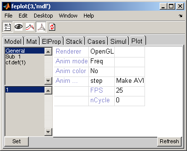
When using fecom ColorDataEval commands (useful when displayed deformation is restituted from reduced deformation at each step), color scaling is updated at each step.
One can use fecom('ScaleColorOne') to force the colorbar scale to remain constant. In that case one can define the limit of the color map with set(cf.ga,'clim',[-1 1]) where cf is a pointer to target feplot figure, and -1 1 can be replaced by color map bondaries.