Contents     Functions              PDF Index

2.2  Identification of modal properties (Id dock)

• Opening and description of used data
• General process
• Importing FRF data
• Write a script to build a transfer structure
• Data acquisition

Identification is the process of estimating a parametric model (poles and modeshapes) that accurately represents measured data. The identification process is typically performed using the dock shown below opened with iicom('dockId').

2.2.1  Opening and description of used data

The following procedure loads data from a .unv file but other way to open and load data are available.

• Open an empty dock iicom('dockid') and load data from the interface by selecting files (see below). A list of acquisition software from which data have been successfully loaded is described in section 2.2.3.
• Reopen a dock previously saved in SDT format (.mat).
  • For saving : in idcom figure, use File:Save, chose the data that need to be saved (all selected by default) and then chose the saving file name.
  • For reloading: execute the command iicom('curveLoad File.mat')
• Load data from variables in the workspace. It is then possible to load data from files directly into variables (see section 2.2.3, which is useful if data customization is required) or to deal with user-built transfers (see section section 2.2.4) and finally pass the result to Id dock.

  % Unv with wire-frame, transfer and poles
  % Open empty dockid get pointer to feplot (cf) and iiplot (ci)
  [ci,cf]=iicom('dockid'); 
  % Build gartid.unv file the first time, then provide file name
  fname=demosdt('build gartid.unv'); 
  % Data are stored into a variable to help you build custom loading procedure
  UFS=ufread(fname); 
  wire=UFS(1); % Test wireframe
  XF=UFS(2); % Transfers
  ID=UFS(3); % List of modes
  cf.mdl=wire; % Store the wireframe in the feplot figure
  % Put transfers to iiplot figure (Transfers named test are the ones 
  ci.Stack{'curve','Test'}=XF; concerned by the current identification)
  ci.Stack{'curve','IdMain'}=ID; % Store the poles in the iiplot figure
  iicom('iix:TestOnly'); % Equivalent to :  idcom figure, tab Stack, 
  % right click on Test and select 'Display selected data'
  

  When manual assignation is performed, do not forget to click on to refresh the tables (for instance the pole list in idcom). Note that to perform identification, only the transfers are needed: the wireframe allows visualizing the identified mode shapes and the list of poles is helpful if previous identification has been performed.

On top of the Test and IdMain data discussed above, other useful data used throughout the identification process and stored in the iiplot Stack are

• Test contains measured frequency response functions. See section 2.2.3 ways to initialize this data set.
• IdFrf contains the synthesis of transfers associated with given set of transfers (shown in red in the figure above).
• IdAlt contains the alternate set of modes (poles and residues). These are listed on the left list of the Ident tab below.
• IdMain contains the main set of modes (poles and residues). These are listed on the right list of the Ident tab.

[ci,cf]=gartid; % Open dockid with stored data and performs identification
ci.Stack % Display list of stored data in the Stack of iiplot

Test=ci.Stack{'curve','Test'}; % Retrieve data from iiplot
IdFrf=ci.Stack{'curve','IdFrf'};
IdMain=ci.Stack{'curve','IdMain'};
IdAlt=ci.Stack{'curve','IdAlt'};

wire=cf.mdl.GetData; % GetData is used to retrieve a copy. 
% Otherwise all modifications are propagated to feplot

Here is a tutorial for interactive data loading in DockId

You will need the garteur example files, which can be found in SDTPath/sdtdemos/gart*.m. If these files are not present, click on the first step on the following tutorial in the HTML version of the documentation or download the patch at the adress https://www.sdtools.com/contrib/garteur.zip and unzip the content in the the folder SDTPath/sdtdemos.

1. Run Execute the command iicom('dockid') to open an empty dock.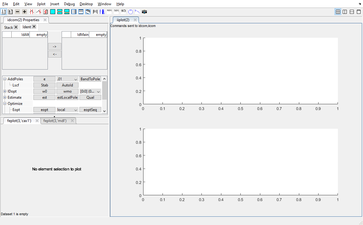

   

   The dock is divided in three parts:

   • At right, the iiplot figure where are displayed all curves (measured transfers, synthesized transfers, mode indicators...)
   • At the top left hand corner, the idcom figure which is used to interact with the data in iiplot, especially here using the Ident tab to perform the identification process
   • At the bottom left hand corner, the feplot figure where the wireframe is displayed. It lets you animate the identified modeshapes. The feplot('mdl') is accessible behind and lets you visualize the information about the wireframe.
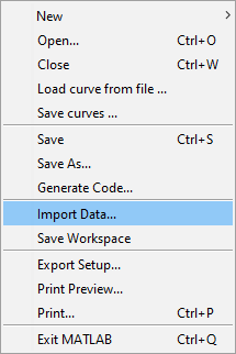
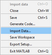
2. Run The loading of .unv files can be realized from iiplot or feplot. Activate for instance the idcom figure and select File:ImportData...

   Here are the 4 possible menus in this order: iiplot, idcom, feplot and feplot('mdl').

   

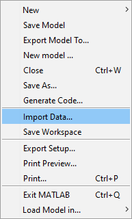
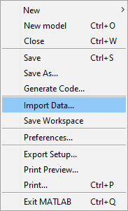
   In the opening window, select the file to load. For this tutorial, the file is located at SDTPath/sdtdemos/gartid.unv.

   Once selected, the Unv tab is displayed in the idcom or the feplot('mdl') figure (depending the chosen menu for ImportData.

   

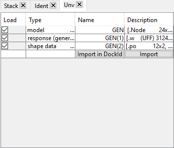
   It shows that three types of data are present in the file: a wireframe, transfers and identified mode shapes. Select the three check boxes to load everything.

3. Run Click on Import (or Import in DockId which is used to build dockId if the loading is performed in a feplot or an iiplot figure outside a dockid).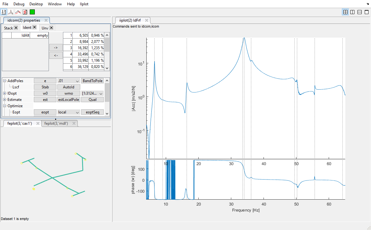

   

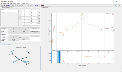
   The data are loaded: transfers are shown in the iiplot figure, the wireframe in the feplot figure and the list of poles in the tab Ident of the idcom figure.

4. Run Once an identification is performed, click on Save in the idcom figure.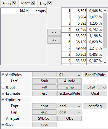

   

   A windows pops-up to ask what data must be saved. Save all (by default) to set all the data and info on the dockid in the saving file.

   Close the dock. A pop-up should appear to ask if you really want to close iiplot (this is to ensure that no data is lost if no saving has been performed), click on Close without saving.

5. Run To reload the saved dock, two possibilities are available:
   • Execute the command iicom('curveload filename')
   • Open an empty iiplot figure and load the saved file with File:Import Data...

2.2.2  General process

The proposed identification process is outlined below. The main steps of the methodology are

• Initial pole estimates are placed in IdAlt using advanced pole picking, LSCF (see section 2.3) or any other algorithm outside SDT.
• A user validated list of poles is kept in IdMain. The arrows between the two list in the interface (which correspond to the ea and er commands) can be used to move poles between the two lists: add missed poles, remove computational or undesired poles .
• Shapes (pole/residue models, residual terms, modeshapes derived from residues) are then estimated for each pole given in IdMain. Several strategies exist and are more deeply explained at section 2.5
  • Broad band estimation on the whole frequency band : est command/button
  • Narrow band estimation on the selected band : estlocal command/button
  • Iterative local estimation around each pole : estlocalpole command/button
• Optimizing poles (and residues) of the current model depending on the quality obtained by the previous passes. As for the estimation of shapes, there three strategies for the optimization:
  • Broad band update : eup for high number of poles and eopt for up to 2-3 poles
  • Narrow band update on the selected band: euplocal and eoptlocal
  • Iterative local updates around each pole: eoptSeq

---

Figure 2.7: Modal identification process with links to corresponding sections

---

This process is handled through the Ident tab opened with iicom('InitIdent') or with the interface by clicking on Tab : Ident from the iiplot or idcom figure.

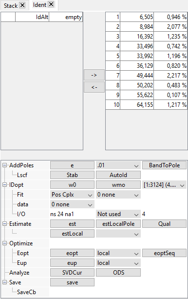
The main steps, associated with level 1 lines in the GUI tree are the topics of specific sections of the documentation:

• AddPoles : use an initial algorithm to estimate poles (single pole estimator or selection in a stabilization diagram LSCF).
• IDopt : select frequency range and possibly define properties of transfers (displacement, velocity, acceleration, MIMO,...)
• Estimate shapes using a frequency domain output error method that builds a model in the pole residue form (see section 5.6). Theoretical details about the underlying algorithm are given in section 2.6.5. Section 2.5.3 addresses its typical shortcomings.
• Adjust poles using one of the non-linear optimization algorithms.
• Transform the output to a format dealing with MIMO constraints, reciprocity, ...

The gartid script gives real data and an identification result for the GARTEUR example. The demo_id script analyses a simple identification example.

2.2.3  Importing FRF data

SDT stores transfer functions in the Response data (.w,.xf fields) or curve (.X,.Y fields) formats. The following table gives a partial list of systems with which the SDT has been successfully interfaced.

• Universal files are easiest if generated by your acquisition system. Writing of an import script defining fields used by SDT is also fairly simple and described below (you can then use ufwrite to generate universal files for export).

  The ufread and ufwrite functions allow conversions between the xf format and files in the Universal File Format which is supported by most measurement systems. A typical call would be

  % generate gartid.unv (or retrieve file name if already generated)
   fname=demosdt('build gartid.unv'); 
   UFS=ufread(fname);  % read the unv file
   UFS % This command display in the command window the content of the file
   xf=UFS(2); % Read the transfers in the file and store in the variable xf
   %% Do everything needed with the data for customization if needed %%%
   % For instance extract channels 1:4
   xf=fe_def('SubDofInd',xf,1:4) 
   % Then pass to iiplot for view and ID purposes
   ci=idcom;   % For identification purposes open IDCOM
   % Store transfers in 'Test' which are transfers to be identified
   ci.Stack{'curve','Test'}=xf; 
  
   % To only view data in figure(11) the following would be sufficient
   cj=iiplot(11);      % open an iiplot in figure 11
   iiplot(cj,UFS(1));  % show UFS(1) there
  

  where you read the database wrapper UFS (see xfopt), initialize the idcom figure, assign dataset 2 of UFS to dataset 'Test' 1 of ci (assuming that dataset two represents frequency response functions of interest).

  Note that some acquisition systems write many universal files for a set of measurements (one file per channel). This is supported by ufread with a stared file name UFS=ufread('FileRoot*.unv');

• Polytec files need many options to extract data (Time/Transfers, Estimator H1/H2, Velocity/Force...). Please read the dedicated polytec documentation to adapt the example below to your needs. Note that the code below needs Polytec File Access to be installed.

   fname=sdtcheck('patchget',struct('fname','PolytecMeas.svd'));
   % Provide a cell array with all readable measured data
   list=polytec('ReadList',fname);
   display(list);
   % Extract the transfer function Vib/Ref1 
   % with the estimator H1 Displacement/Voltage
   RO=struct('pointdomain','FFT','channel','Vib & Ref1',...
   'signal','H1 Displacement / Voltage');
   XF=polytec('ReadSignal',fname,RO);
   % alternative call using one row of the cell array "list"
   XF=polytec('ReadSignal',fname,struct('list',{list(20,:)}));
  

  To avoid the manual filling of the reading options, it is also possible to simply load data from the interface : follow the tutorial in section section 2.2.1) but select the .svd file instead of the .unv file and do right-click+Read selected on the line you want to read. Loaded transfers can then be stored to variables with the command ci=iiplot;xf=ci.Stack{'Test'};

2.2.4  Write a script to build a transfer structure

When writing your own script to transcript data to xfstruct format, you must have a MATLAB structure composed at minimum of the fields

• .w : a column vector of frequencies
• .xf : a matrix of measured frequency responses (one row per frequency, one column per measurement channel).

Other fields may be required to specify the type of data and the type of model to use for identification. Two main optional fields are presented here:

• .dof field can be used to specify the meaning of each transfer (input and output DOF).

  This field should be set for title/legend generation (this is a label).
  For correct display of shapes in feplot, the .dof may be a direct specification of direction in simple cases where the sensors are really oriented in global axes, but in general is just a label for the sensor orientation map stored in a sens.tdof field. See section 2.7 for details on geometry declaration.
  In the example below one considers a MIMO test with 2 inputs and 4 outputs stored as columns of field .xf with the rows corresponding to frequencies stored in field .w. You script will look like

 ci=idcom;
 [XF1,cf]=demosdt('demo2bay xf');% sample data and feplot pointer
 out_dof=[3:6]+.02'; % output dofs for 4 sensors in y direction
 in_dof=[6.02 3.01]; % input dofs for two shakers at nodes 1 and 10
 out_dof=out_dof(:)*ones(1,length(in_dof));
 in_dof=ones(length(out_dof),1)*in_dof(:)';
 XF1=struct('w',XF1.w, ...   % frequencies in Hz
            'xf',XF1.xf, ... % responses (size Nw x (40))
            'dof',[out_dof(:) in_dof(:)]);
 XF1=xfopt('check',XF1);
 ci.Stack{'curve','Test'}=XF1;          % sets data 
 iicom(ci,'submagpha'); % display 
 ci.Stack{'Test'}.idopt % field now points to ci.IDopt
 ci.IDopt.nsna=size(out_dof,1); % Possibly correct number of outputs
 ci.IDopt.recip='mimo';ci.IDopt % Set reciprocity to mimo

 cf.def=ci.Stack{'Test'}; fecom('ch35'); % frequency of first mode

You can check these values in the iicom('InitChannel') tab.

• .idopt field should also be filled for correct identification using id_rc,. For the main data set called Test the .idopt field is that of the figure which is more easily accessed from ci.IDopt. These correspond to the IDopt part of the Ident tab (see section 2.4). You can also edit these values in a script. For correct identification, you should set

 ci=demosdt('demogartid'); 
 ci.IDopt.Residual='3';
 ci.IDopt.DataType='Acc';
 ci.IDopt.Absci='Hz';
 ci.IDopt.PoleU='Hz';
 iicom('wmin 6 40') % sets ci.IDopt.Selected
 ci.IDopt.Fit='Complex';
 ci.IDopt  % display current options

For correct transformations using id_rm, you should also verify ci.IDopt.NSNA (number of sensors/actuators), ci.IDopt.Reciprocity and ci.IDopt.Collocated.

For correct labels using iiplot you should set the abscissa, and ordinate numerator/denominator types in the data base wrapper. You can edit these values using the iiplot properties:channel tab. A typical script would declare frequencies, acceleration, and force using (see list with xfopt _datatype)

 UFS(2).x='Freq';UFS(2).yn='Acc';UFS(2).yd='Load';UFS(2).info

2.2.5  Data acquisition

The SDT does not intend to support the acquisition of test data since tight integration of acquisition hardware and software is mandatory. A number of signal processing tools are gradually being introduced in iiplot (see ii_mmif FFT or fe_curve h1h2). But the current intent is not to use SDT as an acquisition driver. The following example generates transfers from time domain data

frame=fe_curve('Testacq');  % 3 DOF system response
% Time vector in .X field, measurements in .Y columns
frf=fe_curve('h1h2 1',frame); % compute FRF
ci=iicom('Curveid');iicom('curveinit','Test',struct('w',frf.X,'xf',frf.H1))
iicom('SubMagPha');

You can find theoretical information on data acquisition for modal analysis in Refs. [2][3][4][5][6].