
 PDF Index
|
Contents
Functions
PDF Index |

The first step of the model identification (see the whole process at section section 2.2.2) is to build an initial list of poles. This list can be provided from various ways:
In the GUI, algorithms linked to the pole initialization are grouped under AddPoles :
The iteratively refined model is fully characterized by its poles (and the measured data). The initialization of the model optimization process can thus easily be performed from any external modal identification algorithm.
If the external software or script used to perform the identification is able to save the result in the universal file format, simply load it like described in section section 2.2.1.
Else, after storing the measured transfers as a curve named Test in a iiplot figure (see section 2.2.1), add poles with the command
 ci.Stack{'IdMain'}.po =[...
            1.1298e+02   1.0009e-02
            1.6974e+02   1.2615e-02
            2.3190e+02   8.9411e-03];
% ci is the pointer to the iiplot figure containing the Test curve
where the array contains as many lines as poles : the first column provides the pole frequencies in Hz and the second one the pole dampings.
With the list of poles and the measured transfers, you have all you need to recreate an identified model (even if you delete the current one, see section section 2.5) but it also lets you refine the model by adding the line corresponding to a pole that you might have omitted.
The LSCF algorithm is based a rational fraction description of the transfers. The interest of this algorithm is that polynomials are expressed on the base of the z transform which deeply improves the numerical conditioning (often problematic for high order models in the rational fraction form). Moreover, classical stabilization diagram resulting from the identification at various model orders is often very "clean": numerical modes which either compensate noise or residual terms have negative damping and or thus easily removed from the diagram.
The following tutorial describes how to initialize the poles using the LSCF algorithm.
 Run
Execute the command iicom('dockid') to open an empty dock and load the wireframe and the transfers contained in the file SDTPath/sdtdemos/gartid.unv (Do not load the identification result because it will be performed in the following).
See section 2.2.1 for the data loading procedure, or just click on Run in the html version of the documentation.
Run
Execute the command iicom('dockid') to open an empty dock and load the wireframe and the transfers contained in the file SDTPath/sdtdemos/gartid.unv (Do not load the identification result because it will be performed in the following).
See section 2.2.1 for the data loading procedure, or just click on Run in the html version of the documentation.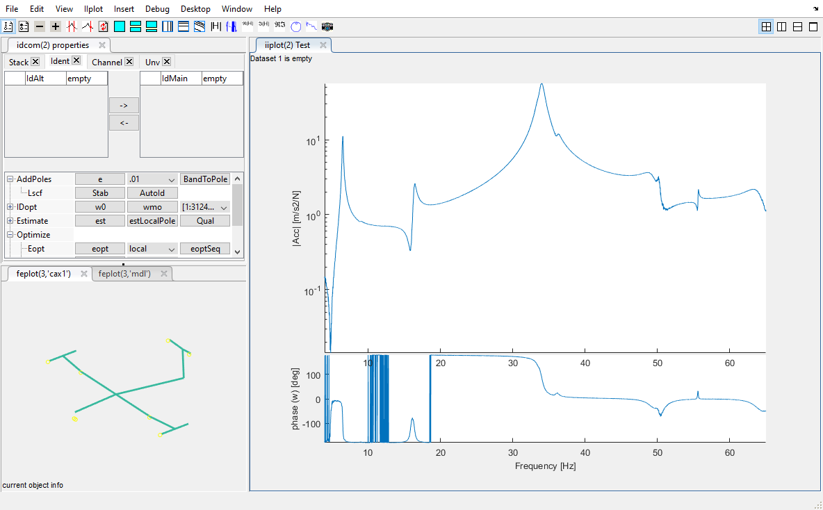
Run
In the tab Ident, click on the button Stab to open the Tab StabD which allows interaction with the stabilization diagram built with the LSCF algorithm.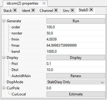
The button AutoId open this StabD tab and directly performs diagram building and pole extraction with default values of the algorithm. It is often useful for a quick evaluation.
Run
The StabD tab contains options to build the stabilization diagram in the sub-list under Generate :
The building of a stabilization diagram with a maximum order of 100 is not very costly and should be used for most applications. We advise then to estimate the total number of poles in the whole band of interest (fmax-fmin), to divide this total bandwidth by this number and to multiply the result by 5 in order to find the band width which contains in average 5 expected modes (20 times less than the maximum model order).
In our test case, we attempt to find 12 modes in a total bandwidth of 60Hz) : set the band parameter to 60/12*5=25 Hz.
Run
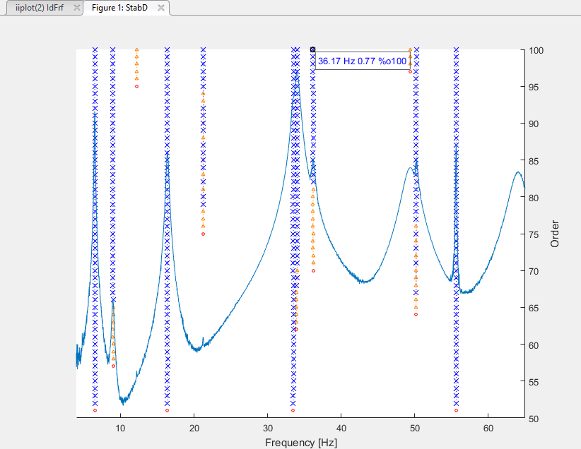
Click on Generate to build the stabilization diagramm.In the diagram, the status of the poles are marked by
Frequency and damping stability are defined by the parameters Ftol and Dtol under the sub-list Display. If relative frequency or damping of poles from consecutive model orders are below the parameter values (in %), they are considered stable.
In presence of very clean measurements of a very strictly linear system, these values could be more restrictive. In the opposite, they should be increase for noisier data and/or in presence of small non-linearities. When the values of Ftol and Dtol are modified, click on Display to refresh the diagram.
To improve the analysis of the stabilization diagram, mode estimators can be displayed on top of it : the list of all available mode estimators at the right of DispMode (see ii_mmif for details)
The stabilization diagram displayed with the logSumI mode estimator leads to this picture.
Run
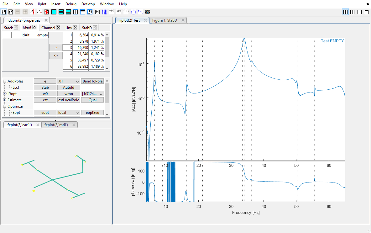
To automatically extract all stabilized poles (with a blue cross at the last model order), click on Renew at the line AutoIdMain. The button specifies "Renew" because all current poles in the fmin - fmax band will be deleted and replaced by the extracted ones from the diagram.The extracted poles are displayed at the right table of the tab Ident. On the transfers, pole locations are specified by the vertical lines.
Run
Back to the stabilization diagram, two columns are started but not stabilized around 12Hz and 50Hz. For the column at 12Hz, the logSumI indicator shows almost no resonance. For the column at 50Hz, the resonance is well visible but more damped than the close mode.To evaluate the pertinence of the poles despite that they do not fully satisfy the stabilization criteria, click on the icon  and select the last order of the column.
In the StabD tab, click on Estimate at the line CurLocal. This action performs a local estimation with the selected pole around its frequency. The channel presenting the highest contribution for this mode is automatically selected and the synthesized transfer is superposed to the measurement.
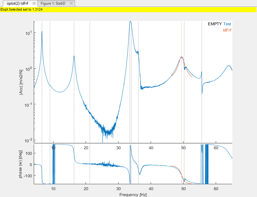
The synthesized transfer does not exactly fit the measurements (which is very noisy around this frequency) but is enough representative to be selected as initial pole prior to optimization.
Run
The pole used to perform the local estimation is stored in the left table of the tab Ident : the list of the alternate poles. Because it is representative enough to describe the mode, it can be added to the list of main poles (the right table) by clicking on the arrow.Do the same for the not stabilized column around 12Hz. The result is much more doubtful because the mode is almost not visible and the measurement very noisy. More over the local estimation does not fit very well. Nevertheless, add this pole to the main list: we will analyze its pertinence in the following using Quality criteria and trying to optimize it.
Finally, the mode estimator on top of the stabilization diagram shows that a mode at the right of the frequency band is probably there but not identified by the LSCF algorithm. This case can be handled by manually adding a pole using the single pole estimator.
Because getting an initial estimate of the poles of the model is the often tedious, algorithms like LSCF or other broadband algorithms are very helpful to quickly extract most of the poles: dynamic responses of structures typically show lightly damped resonances which are most of the time well detected. Nevertheless, using such algorithm often leads to two issues that need to be handled:
To deal with missing poles, the easiest way to enrich the initial estimate of the poles is to use a narrow band single pole estimation near considered resonances of the response or minima of the Multivariate Mode Indicator function (use iicom Showmmi and see ii_mmif for a full list of mode indicator functions).
The idcom e command (based on a call to the ii_poest function) lets you to indicate a frequency (with the mouse or by giving a frequency value) and seeks a single pole narrow band model near this frequency (the pole is stored in ci.Stack{'IdAlt'}. Once the estimate found, the iiplot drawing axes are updated to overlay ci.Stack{'Test'} (the measured transfers) and ci.Stack{'IdFrf'} (the narrow band transfer synthesis).
In the plot shown above the fit is clearly quite good. This can also be judged by the information displayed by ii_poest
 LinLS:  1.563e-11, LogLS  8.974e-05, nw 10
 mean(relE) 0.00, scatter 0.00
 Found pole at 1.1299e+02   9.9994e-03
which indicates the linear and quadratic costs in the narrow frequency band used to find the pole, the number of points in the band, the mean relative error (norm of difference between test and model over norm of response which should be below 0.1), and the level of scatter (norm of real part over norm of residues, which should be small if the structure is close to having modal damping).
If you have a good fit and the pole differs from poles already in your current model, you can add the estimated pole (add poles in ci.Stack{'IdAlt'} to those in ci.Stack{'IdMain'}) using the idcom ea command (or the associated button : arrow pointing to the right). If the fit is not appropriate you can change the number of selected points/bandwidth and/or the central frequency.
Remark : In the interface or using idcom e command, an initial guess of the damping value is used to search for the local mode. The algorithm sometimes fails if this value is too far from the real damping.
In rare cases where the local pole estimate does not give appropriate results you can add a pole by just indicating its frequency (f command) or you can use the polynomial (id_poly), direct system parameter (id_dspi), or any other identification algorithm to find your poles. You can also consider the idcom find command which uses the MMIF to seek poles that are present in your data but not in ci.Stack{'IdMain'}.
To deal with cases where you have added too many poles to your current model, use the idcom er (or the associated button : arrow pointing to the left) command to remove certain poles.
This phase of the identification relies heavily on user involvement. You are expected to visualize the different FRFs (use the +/- buttons/keys), check different frequency bands (zoom with the mouse and use iicom w commands), use Bode, Nyquist, MMIF, etc. (see iicom Show commands). The iiplot graphical user interface was designed to help you in this process and you should learn how to use it (you can get started in section 2.1).
gartid % Open interface with gartid demo
idcom('e .1 6')

%idcom('Est 0.1 6.0000); % does click
%LinLS:  2.110e+02, LogLS        Inf, nw 63
% mean(relE) 0.03, scatter 0.16 : good
%Found pole at 6.4901e+00   8.7036e-03
Let's go back to the previous tutorial to add the missing pole at the end of the frequency band.
If you have not performed previous tutorial (or if you closed everything at the end), click on this link
in the HTML version of the documentation to get ready for the following.
Run
Click on the button e in the tab Ident. Then click approximatively at the location of the resonance to start the single estimation algorithm at that frequency. Please note that, especially in presence of very lightly damped structure, it is sometimes necessary to edit the value of the expected damping in the list on the right of the button e for the algorithm to find the correct pole.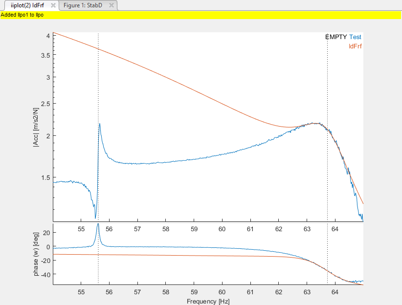
The fit is correct at the resonance: add the pole to the main list by clicking on the arrow −>
A procedure allowing to add several poles by dragging the mouse to select a band for the single pole estimator will be implemented in further release. Currently the procedure only takes the maximum of the band and does not estimate damping.
(Obsolete) A class of identification algorithms makes a direct use of the second order parameterization. Although the general methodology introduced in previous sections was shown to be more efficient in general, the use of such algorithms may still be interesting for first-cut analyses. A major drawback of second order algorithms is that they fail to consider residual terms.
The algorithm proposed in id_dspi is derived from the direct system parameter identification algorithm introduced in Ref. [7]. Constraining the model to have the second-order form
| (2.1) |
it clearly appears that for known [cT], {yT}, {uT} the system matrices [CT], [KT], and [bT] can be found as solutions of a linear least-squares problem.
For a given output frequency response {yT}=xout and input frequency content {uT}=xin, id_dspi determines an optimal output shape matrix [cT] and solves the least squares problem for [CT], [KT], and [bT]. The results are given as a state-space model of the form
| (2.2) |
The frequency content of the input {u} has a strong influence on the results obtained with id_dspi. Quite often it is efficient to use it as a weighting, rather than using a white input (column of ones) in which case the columns of {y} are the transfer functions.
As no conditions are imposed on the reciprocity (symmetry) of the system matrices [CT] and [KT] and input/output shape matrices, the results of the algorithm are not directly related to the normal mode models identified by the general method. Results obtained by this method are thus not directly applicable to the prediction problems treated in section 2.8.2.
(Obsolete) Among other parameterizations used for identification purposes, polynomial representations of transfer functions (5.31) have been investigated in more detail. However for structures with a number of lightly damped poles, numerical conditioning is often a problem. These problems are less acute when using orthogonal polynomials as proposed in Ref. [8]. This orthogonal polynomial method is implemented in id_poly, which is meant as a flexible tool for initial analyses of frequency response functions. This function is available as idcom poly command.


