PDF Index
|
Contents
Functions
PDF Index |
Once a model is created (you have estimated a set of poles in IdMain), the residues need to be computed. The classical way to do so in the litterature is to determine residues on the whole frequency band for the synthesized FRFs stored in ci.Stack{'IdFrf'} to be as close as possible to the measured data in the least square sense. This strategy and others using narrow bands are detailed in section section 2.5.1.
To analyze the quality of the identification, several criteria definined by mode and by transfer have been developped to help navigate through the data. The quality table and its analysis are described in section section 2.5.2.
A non exhaustive list of classical issues using the id_rc algorithm is given in section section 2.5.3.
The standard estimation of residues on the whole frequency band is performed with the command idcom est (or the equivalent button in the interface).
This method can give good results if the measurements are very clean and the system very close to a perfectly linear system. If noise, non-linear distorsion badly identified pole is present at some frequency bands, especially if it worresponds to high amplitudes in the transfers, fitting all modes together on the whole frequency band can engender strong bias in the identification of residue with low amplitude.
In this case, and if a broadband model is not necessary, it is most of the time preferable to perform a sequential identification with a narrow band arround each mode to extract the residuals. This is automaticaly achived using the command idcom estlocalpole (or the equivalent button in the interface).
An alternative way to handle these problems of bias for some modes is to perform local identifications which update residues only on a smaller working frequency band. To do so, you need to select a close frequency band inside which the residues are poorly identified with the button  and then use the command idcom estlocal (or the equivalent button in the interface).
To highlight the differences between these strategies, the following tutorial uses the GARTEUR test case with the initial poles identified in the previous section section 2.3.
 Run
Click on the link in the HMTL version to initialize the tutorial. Else, execute the command sdtweb('_tuto','gartid') to open the list of tutorials and execute the first step of the tutorial Estimate.Run
In the Ident tab, click on the button est to identify the residues using the broadband method.
Run
Click on the link in the HMTL version to initialize the tutorial. Else, execute the command sdtweb('_tuto','gartid') to open the list of tutorials and execute the first step of the tutorial Estimate.Run
In the Ident tab, click on the button est to identify the residues using the broadband method.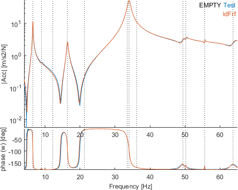
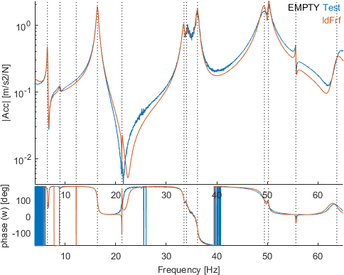
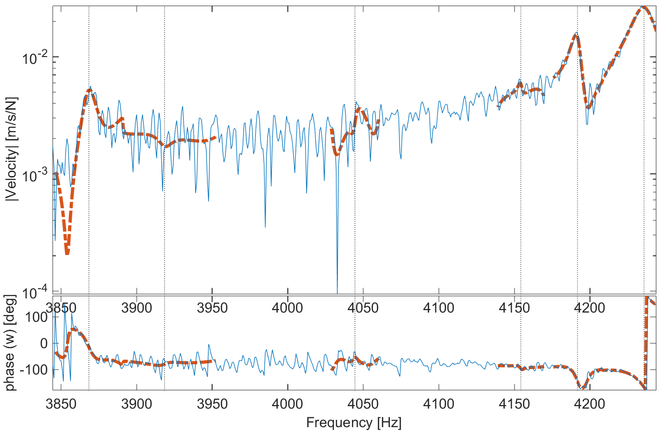
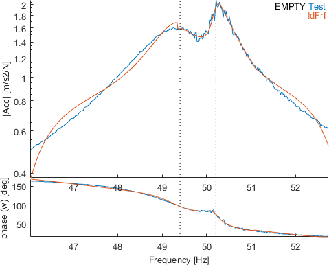
For some transfers the superposition seems quite good like for the first figure whereas it is clearly bad for many modes for some others like the second figure.
Run
In the Ident tab, click on the button estLocalPole to identify the residues using the sequential narrowband method.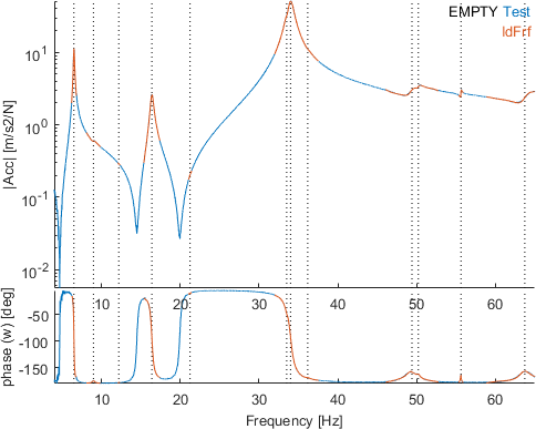
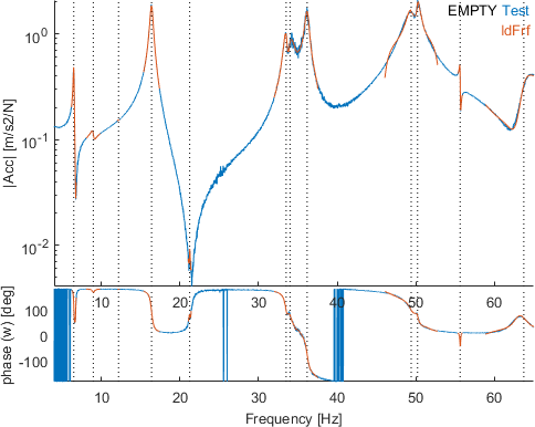
Each local identification is clearly closer to the measurements than using the broadband strategy. It should be noted that residues correspond to mode shapes and that consequences on proper identification of shapes can be important. The figure below shows the MAC between the set of mode shapes obtained with the est versus the estLocalPole algorithms.
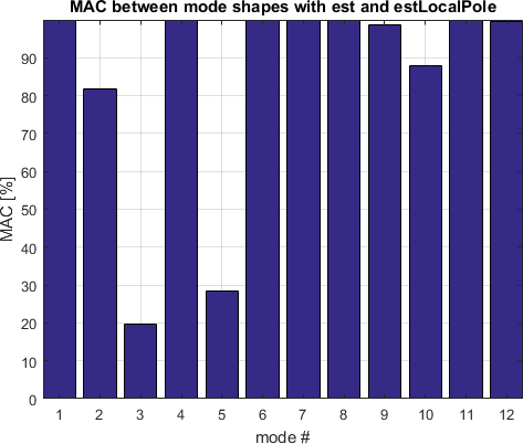
The two modes 3 and 5 which are very less excited (the physical meaning of these poles is even still question for the moment) are very impacted. Modes 2 which is less excited is quite different. Mode 10 is well visible but the pole seems badly identified as shown on the figure below (zoom on modes 9 and 10) : the residues are differently biased to compensate in the two strategies.
The need to add/remove poles is determined by careful examination of the match between the test data ci.Stack{'Test'} and identified model ci.Stack{'IdFrf'}. For a very small amount of data, you could take the time to scan through different sensors, look at amplitude, phase, Nyquist, ... but when the number of sensors and the number of modes become high, the manual scanning is too much time consuming.
Too help navigate through a large amount of data to efficiently analyze the quality of the measurements, several criteria have be defined and can be used to sort sensors by mode. In the following, each pair of sensor/actuator corresponding to a column of the measured transfers HTest associated to a column of the synthesized transfers Hid will be indexed by c.
A perfect identification is obtained if measured and synthesized transfers are perfectly superposed. Because the contribution of a mode is characterized by the fact that its amplitude is maximum around the resonance frequency, a classical method to analyze the quality of the fit is to compare the measurement and the identification around each mode. We thus define the identification error for a mode j and input/output pair c by
| (2.3) |
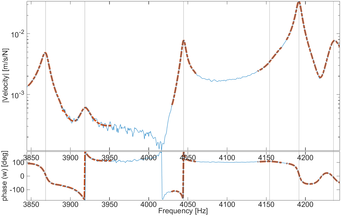
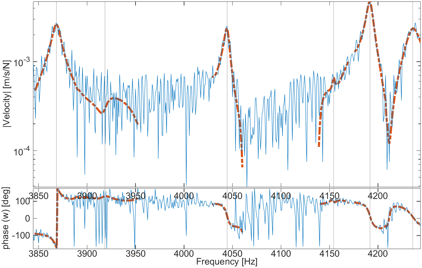
with ωj the modal frequency and ζj the modal damping. α is a scale factor of the frequency bandwidth, with α=1 corresponding to the classical bandwidth at -3dB and α=5, a pertinent value used here. This error criterion can be seen as a numerical evaluation of the quality of the historical "circle fit" method. The figure 2.9 shows a simple case on the mode at 4050Hz. On the left, the measurement in blue line is noisy so that the correspondence with the identification in red dotted line is not good. This is coherent with the value of the error criterion evaluated at 30%. On the right, the resonance of the mode is well visible and the superposition with the identification is almost perfect. This visual analysis is well confirmed by the error criterion evaluated at 0.4%
For most applications, high error is expected close to vibration nodes where the observability is weak. To avoid taking into account such transfers as badly identified, the level criterion for a given mode j and a given sensor/actuator pair c is defined as the ratio between the quadratic mean for the channel c around the resonance and the maximum quadratic mean on all the channels.
| (2.4) |
Problematic sensors are those presenting a high error despite a significant level. Thus, considering the error criterion and the level criterion is often not appropriate. A new criterion called Noise Over Signal (NOS) is obtained by multiplying both criteria together
| (2.5) |
in order to highlight transfers where high error is associated to a un level, and thus critical. For a reasonable identification, the approximation made on (2.5) use the fact that HTest,c et HId,c should be close and so that
∫ωj(1−αζj)ωj(1+αζj)|HTest,c(s)|2 / ∫ωj(1−αζj)ωj(1+αζj)|Hid,c(s)|2≈ 1. This approximation illustrate that the product ej,c× Lj,c is close to the ratio of the identification error (hence a estimation of the noise) over the maximum response (hence the signal level), which explains the origin of the NOS terminology.
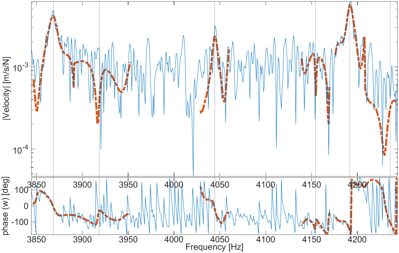
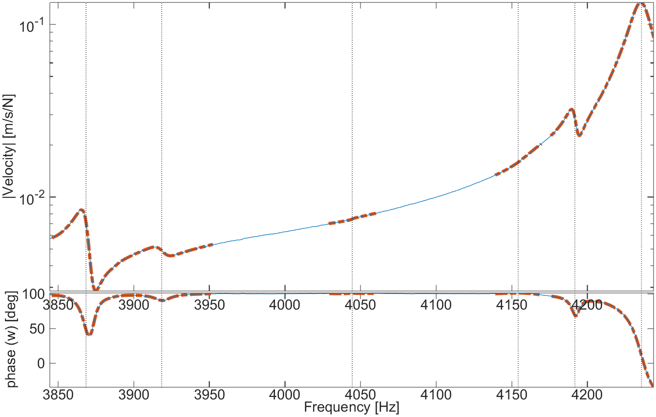
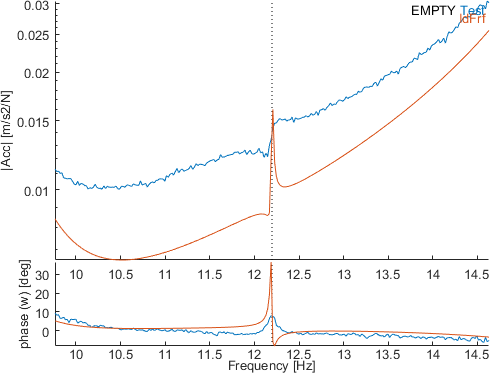
The figure 2.10 (first) shows an example of a transfer function with a high NOS value (8.3%) : the error is very high at 40.4% whereas the level is still significant at 20.5%. The mode is very badly identified (barely visible on this transfer) but the amplitude of the identified residue is important for the definition of the mode shape. The existence of sensor/actuator pairs with high noise level at high amplitude, highlighted by NOS, is typical of weekly excited modes (the controllability is weak for the chosen excitation location). On the second image, the transfer function also shows a high NOS value (24.7%) and a high error (24.7%) but graphically, the mode is very visible. The high NOS value is here due to a bad identification of the pole, which induces a bias in the residue to compensate. This second example illustrates that this criterion is also well adapted to the detection of problems of coherence between measurements (different settings between measurement systems, behavior evolution of the system during measurement,...).
After manual analysis of many measurements, two intermediate cases are often found: the measurement is noisy but still has a sufficient contribution to be identified with confidence or the contribution of a mode is so weak that it cannot be separated from other modes without raising questions on a more or less important estimation bias. To distinguish the two cases, a last contribution criterion is introduced
| (2.6) |
to measure the modal contribution of a specific mode j relatively to the global response of all the other modes around its resonance frequency, thus giving an indication of its visibility (Hid,j,c is the transfer synthesis containing only the mode j). For highly noisy transfer functions, this indicator can be negative and is then set to 0.
Figure 2.11 shows transfer functions for which this kind of question is raised. On the first image, around 4050Hz, the mode is well visible despite a relatively high noise level. It could be useful to keep this channel to well interpret the correlation. On the second image, a transfer function is shown where the error is very low but for which the resonance of the considered mode is not visible at all. The capacity to identify the residue with confidence is low because the identification could clearly be significantly biased
Proposed criteria allow decomposing identification error sources in contributions by mode and by transfer function (sensor/actuator pair). For each mode, clearly problematic sensors showing high error with low contribution and a low level can be automatically discarded and only results properly identified can be kept with a high confidence on the quality.
Intermediate results can be analyzed in more details using sorting by level, contribution or NOS to highlight problematic transfer functions, as illustrated in the following tutorial.
Let's go back to the previous tutorial. If you have not performed it (or if you closed everything at the end), click on this link
in the HTML version of the documentation to get ready for the following.
Run
In the Ident tab, click on est to perform an broad band identification of the residues. Click then on the button Qual to open the tab Qual which synthesizes all the quality criteria defined above.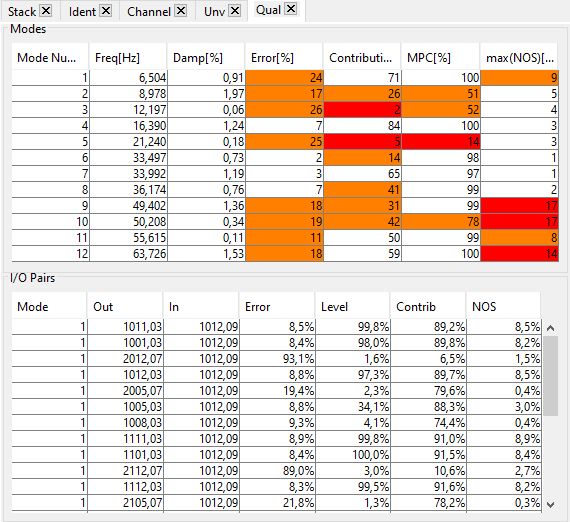
The identification quality is globaly poor, with a mean error quite high arround most modes. Two modes show a very low mean contribution (3 and 5), four modes show a bad MPC whereas expected modes are real (2,3,5 and 10) and finally, three modes present a high max(NOS) (9 10 and 12).
Clicking on a line of the first table Modes updates the second table I/O Pairs with the four quality criteria on all sensors for the selected mode. Each criterion can be sorted by clicking on the corresponding column header and clicking on a line perfoms a zoom on the corresponding transfer arround the mode frequency.
This way, we can for example easily zoom on the transfer with the highest contribution for the mode 3 and the transfer with the highest NOS for the mode 10 :
This highlight the bias in the identification of the residues.
Run
Now click in the Ident tab on estlocalpole to perform a sequential identification by mode with the same poles and click again on Qual to update the Qual tab.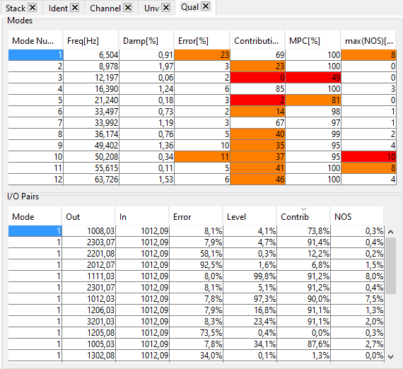
The identification quality is clearly better than using the brodband strategy : mean error is improved everywhere. Nevertheless, modes 3 and 5 still show very low contribution and MPC and mode 10 presents a lower but still high max(NOS).
The zoom on the transfer with the highest contribution for the mode 3 and the transfer with the highest NOS for the mode 10 can again be displayed :
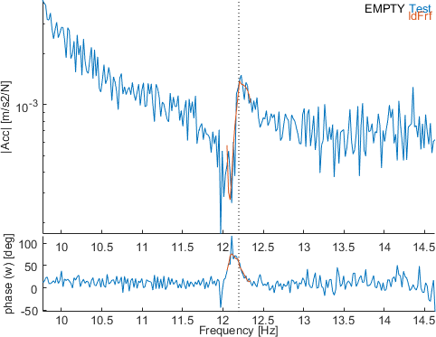
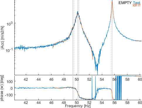
For mode 3, the resonance is not very visible and the measurement very noisy : this mode is probably not well enough excited and is moreover visible very locally (2 sensors higher than 1% contibution). For mode 10, the high NOS do not highlight bad identification anymore (measurement and synthesis are quite well superposed) but shows that the error due to the high measurement noise is present even at sensors where the mode has a high level : a better excitation of the mode should reduce the noise and improve the identification quality.
At this step, quality has been evaluated but we are aware that identified poles are possibly biased. Indeed, the strategy of extraction of poles does not use the exact same model than the one used as a second stage to identify the residues. Non-linear optimization of this initial state should be performed and the impact of this optimization on the identification quality is analyzed in Section section 2.6
This section gives a few examples of cases where a direct use of id_rc gave poor results. The proposed solutions may give you hints on what to look for if you encounter a particular problem.
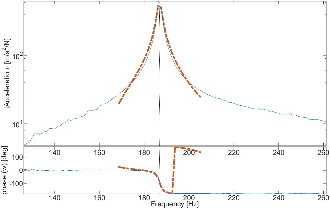
In many cases frequencies of estimated FRFs go down to zero. The first few points in these estimates generally show very large errors which can be attributed to both signal processing errors and sensor limitations. The figure above, shows a typical case where the first few points are in error by orders of magnitude. Of two models with the same poles, the one that keeps the low frequency erroneous points (- — -) has a very large error while a model truncating the low frequency range (- - -) gives an extremely accurate fit of the data (—).
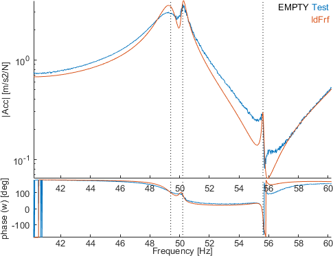
The fact that appropriate residual terms are needed to obtain good results can have significant effects. The figure above shows a typical problem where the identification is performed in the band indicated by the two vertical solid lines. When using the 7 poles of the band, two modes above the selected band have a strong contribution so that the fit (- - -) is poor and shows peaks that are more apparent than needed (in the 900-1100 Hz range the FRF should look flat). When the two modes just above the band are introduced, the fit becomes almost perfect (- — -) (only visible near 750 Hz).
Keeping out of band modes when doing narrow band pole updates is thus quite important. You may also consider identifying groups of modes by doing sequential identifications for segments of your test frequency band [9].
The example below shows a related effect. A very significant improvement is obtained when doing the estimation while removing the first peak from the band. In this case the problem is actually linked to measurement noise on this first peak (the Nyquist plot shown in the lower left corner is far from the theoretical circle).
Other problems are linked to poor test results. Typical sources of difficulties are