PDF Index
|
Contents
Functions
PDF Index |
Before actually taking measurements, it is good practice to prepare a wire frame-display (section 2.2.1 and section 4.1.1 for other examples) and define the sensor configuration (section 2.2.2).
The information is typically saved in a specific .m file which should look like the gartte demo without the various plot commands. The d_pre demo also talks about test preparation.
A wire-frame model is composed of node and connectivity declarations.
Starting from scratch (if you have not imported your geometry from universal files). You can declare nodes and wire frame lines using the fecom Add editors. Test wire frames are simply groups of beam1 elements with an EGID set to -1. For example in the two bay truss (see section 4.1.1)
 cf=feplot;cf.model='reset';
 % fecom('AddNode') would open a dialog box
 fecom('AddNode',[0 1 0; 0 0 0]); % add nodes giving coordinates
 fecom('AddNode',[3  1 1 0;4  1 0 0]); % NodeId and xyz
 fecom('AddNode',[5      0 0 0    2 0 0;
                  6      0 0 0    2 1 0]);
 % fecom('AddLine') would add cursor to pick line (see below)
 fecom('AddLine',[1 3 2 4 3]);  % continuous line in first group
 fecom('AddLine',[3 6 0 6 5 0 4 5 0 4 6]); % 0 for discontinuities
 fecom('Curtab:Model','Edit')
 %fecom('save')  % will let you save the model to a mat file
 feutilb('write',cf.mdl) % generates a script
Note that
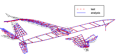
The feplot and fecom functions provide a number of tools that are designed to help in visualizing test results. You should take the time to go through the gartid, gartte and gartco demos to learn more about them.
The geometry declaration defines fields .Node and .Elt. The next step is to declare sensors. Once a sensor configuration defined and consistent with input/output pair declarations in measurements (see section 2.1.4), you can directly animate measured shapes (called Operational Deflection Shapes) as detailed in section 2.2.4. Except for roving hammer tests, the number of input locations is usually small and only used for MIMO identification (see section 2.4).
In the basic configuration with translation sensors, sensor declaration is simply done with a .tdof field. Acceptable forms are
The definition of sensors trough a .tdof field is the simplest configuration. For more general setups, see section 4.6 for sensor definitions and section 4.6.4 for topology correlation.
For interpolation of unmeasured DOFs see section 3.3.2.
The following illustrates the first two forms
TEST=demosdt('DemoGartteWire');

% simply give DOFs (as a column vector)
TEST.tdof = [1011.03 1001.03 2012.07 1012.03 2005.07 1005.03 1008.03  ...
 1111.03 1101.03 2112.07 1112.03 2105.07 1105.03 1108.03 1201.07 ...
 2201.08 3201.03 1206.03 1205.08 1302.08 2301.07 1301.03 2303.07 1303.03]';

% Transfor to 5 column format, which allow arbitrary orientation
TEST.tdof=fe_sens('tdof',TEST);TEST.tdof

feplot(TEST) % With a .tdof field, a SensDof,Test is defined automatically
fecom('curtab Cases','Test');fecom('ProViewOn')


% You can now display FRFs or modes using
 ci=iicom('curveload gartid'); % load data
 fecom(';ProviewOff;Showline')
% Display FRF
cf.def=ci.Stack{'Test'}; % automatically uses sensor definition 'Test'
% Identify and display mode
idcom('e .05 6.5')
cf.def=ci.Stack{'IdAlt'}; % automatically uses sensor definition 'Test'
This new example, mixes all 3 forms
cf=demosdt('demogartteplot') % Load data

% simply give DOFs
cf.mdl=fe_case(cf.mdl,'sensdof','Test', ...
[1011.03 1001.03 2012.07 1012.03 2005.07 1005.03 1008.03 ...
1111.03 1101.03 2112.07 1112.03 2105.07 1105.03 1108.03 1201.07]');

% Give DOF defined in a local basis
cf.mdl=fe_case(cf.mdl,'sensdof append','Test', ...
[2201.01 1; 3201.03 0; 1206.03 0; 1205.01 1; 1302.01 1]);

% Give identifier, node and measurement direction
cf.mdl=fe_case(cf.mdl,'sensdof append','Test', ...
[1 2301 -1 0 0; 2 1301 0 0 1; 3 2303 -1 0 0; 4 1303 0 0 1]);
fecom('curtab Cases','Test');fecom('ProViewOn')
It is also fairly common to glue sensors normal to a surface. The sensor array table (see section 4.6.2) is the easiest approach for this objective since it allows mixing global, normal, triax, laser, ... sensors. The following example shows how this can also be done by hand how to obtain normals to a volume and use them to define sensors.
% This is an advanced code sample
model=demosdt('demo ubeam');

MAP=feutil('getnormal node MAP',model.Node, ...
  feutil('selelt selface',model)); % select outer boundary for normal

i1=ismember(MAP.ID,[360 365 327 137]); % nodes where sensors are placed
MAP.ID=MAP.ID(i1);MAP.normal=MAP.normal(i1,:);
model=fe_case(model,'sensdof','test', ...
  [(1:length(MAP.ID))' MAP.ID MAP.normal]);

% display the mesh and sensors
cf=clean_get_uf('feplotcf',model);
cf.sel(1)='groupall';cf.sel(2)='-test';
cf.o(1)={'sel2ty7','edgecolor','r','linewidth',2}
The SDT does not intend to support the acquisition of test data since tight integration of acquisition hardware and software is mandatory. A number of signal processing tools are gradually being introduced in iiplot (see ii_mmif FFT or fe_curve h1h2). But the current intent is not to use SDT as an acquisition driver. The following example generates transfers from time domain data
frame=fe_curve('Testacq');  % 3 DOF system response
% Time vector in .X field, measurements in .Y columns
frf=fe_curve('h1h2 1',frame); % compute FRF
ci=iicom('Curveid');ci.Stack{'Test'}.w=frf.X; ci.Stack{'Test'}.xf=frf.H1;
iicom('Sub');
You can find theoretical information on data acquisition for modal analysis in Refs. [2][3][4][5][6].
Import procedures are described in section 2.1.4. The following table gives a partial list of systems with which the SDT has been successfully interfaced.
| Vendor | Procedure used |
Bruel & Kjaer | Export data from Pulse to the UFF and read into SDT with ufread or use the Bridge To Matlab software and pulse2sdt. |
| Dactron | Export data from RT-Pro software to the UFF. Use the Active-X API to drive the Photon from MATLAB see photon. |
| LMS | Export data from LMS CADA-X to UFF. |
| MathWorks | Use Data Acquisition and Signal Processing toolboxes to estimate FRFs and create a script to fill in SDT information (see section 2.1.4). |
| MTS | Export data from IDEAS-Pro software to UFF. |
| Polytec | Export data from PSV software to UFF. |
| Spectral Dynamics | Create a Matlab script to format data from SigLab to SDT format. |
Operational Deflection Shapes is a generic name used to designate the spatial relation of forced vibration measured at two or more sensors. Time responses of simultaneously acquired measurements, frequency responses to a possibly unknown input, transfer functions, transmissibilities, ... are example of ODS.
When the response is known at global DOFs no specific information is needed to relate node motion and measurements. Thus any deformation with DOFs will be acceptable. The two basic displays are a wire-frame defined as a FEM model or a wire-frame defined as a SensDof entry.
 % A wire frame and Identification results
 [TEST,IdMain]=demosdt('DemoGartteWire')
 cf=feplot(TEST);   % wire frame
 cf.def=IdMain;     % to fill .dof field see sdtweb('diiplot#xfread')
 % or the low level call : cf.def={IdMain.res.',IdMain.dof,IdMain.po}

 % Sensors in a model and identification results
 cf=demosdt('demo gartfeplot'); % load FEM
 TEST=demosdt('demo garttewire');  % see sdtweb('pre#presen')
 cf.mdl=fe_case(cf.mdl,'sensdof','outputs',TEST)

 cf.sel='-outputs';  % Build a selection that displays the wire frame
 cf.def=IdMain;      % Display motion on sensors

 fecom('curtab Plot');
When the response is known at sensors that need to be combined (non global directions, non-orthogonal measurements, ...) a SensDof entry must really be defined.
When displaying responses with iiplot and a test geometry with feplot, iiplot supports an ODS cursor. Run demosdt('DemoGartteOds') then open the context menu associated with any iiplot axis and select ODS Cursor. The deflection show in the feplot figure will change as you move the cursor in the iiplot window.
More generally, you can use fecom InitDef commands to display any shape as soon as you have a defined geometry and a response at DOFs. The Deformations tab of the feplot properties figure then lets you select deformations within a set.
 [cf,ci]=demosdt('DemoGartteOds')
 cf.def=ci.Stack{'Test'};
 % or the low level call :
 % cf.def={ci.Stack{'Test'}.xf,ci.Stack{'Test'}.dof,ci.Stack{'Test'}.w}
 fecom('CurTab Plot');
You can also display the actual measurements as arrows using
cf.sens=ci.Stack{'Test'}.dof; fecom ShowArrow; fecom scc1;
For a tutorial on the use of feplot see section 4.4.