PDF Index
|
Contents
Functions
PDF Index |
iiplot is the response viewer used by SDT. It is essential for the identification procedures but can also be used to visualize FEM simulation results.
As detailed in section 2.3, identification problems should be solved using the standard commands for identification provided in idcom while running the iiplot interface for data visualization. To perform an identification correctly, you need to have some familiarity with the interface and in particular with the iicom commands that let you modify what you display.
For simple data viewing you can open an iiplot figure using ci=iiplot (or ci=iiplot(2) to specify a figure number). For identification routines you should use ci=idcom (standard datasets are then used see section 2.3).
To familiarize yourself with the iiplot interface, run demosdt('demogartidpro'). Which opens the iiplot figure and the associated iiplot(2) properties figure whose tabs are detailed in the following sections.
 | Toggles the display or not of the iiplot property figure. |
 | Previous channel/deformation, see iicom ch+. |
 | Next channel/deformation. |
 | Fixed zoom on FRF, see iicom wmin. Note that the variable zoom (drag box) is always active, see iimouse zoom. |
 | Start cursor, see iimouse Cursor. |
 | Refresh the displayed axes. |
 | No subplot. See iicom Sub[1,1]. |
 | 2 subplots. See iicom Sub[2,1]. |
 | Amplitude and phase subplots. See iicom Submagpha. |
 | switch lin/log scale for x axis. See iicom xlin. |
 | switch lin/log scale for y axis. See iicom ylog. |
 | switch lin/log scale for z axis. See iicom xlog. |
 | Show absolute value. See iicom Showabs. |
 | Show phase. See iicom Showpha. |
 | Show real part. See iicom Showrea. |
 | Show imaginary part. See iicom Showima. |
 | Show real and imaginary part. See iicom Showr&i. |
 | Show Nyquist diagram. See iicom Shownyq. |
 | Show unwrapped phase. See iicom Showphu. |
 | Snapshot. See iicom ImWrite |
Mouse and keypress operations are handled by iimouse within iiplot, feplot, and ii_mac figures. For a list of active keys press ? in the current figure.
Drag your mouse on the plot to select a region of interest and see how you directly zoom to this region. Double click on the same plot to go back to the initial zoom. On some platforms the double click is sensitive to speed and you may need to type the i key with the axis of interest active. An axis becomes active when you click on it.
Open the ContextMenu associated with any axis (click anywhere in the axis using the right mouse button), select Cursor, and see how you have a vertical cursor giving information about data in the axis. To stop the cursor use a right click or press the c key. Note how the left click gives you detailed information on the current point or the left click history. In iiplot you can for example use that to measure distances.
Click on pole lines (vertical dotted lines) and FRFs and see how additional information on what you just clicked on is given. You can hide the info area by clicking on it.
The axes ContextMenu (click on the axis using the right mouse button) lets you select , set axes title options, set pole line defaults, ...
The line ContextMenu lets you can set line type, width, color ...
The title/label ContextMenu lets you move, delete, edit ... the text
After running through these steps, you should master the basics of the iiplot interface. To learn more, you should take time to see which commands are available by reading the Reference sections for iicom (general list of commands for plot manipulations), iimouse (mouse and key press support for SDT and non SDT figures), iiplot (standard plots derived from FRFs and test results that are supported).
iiplot considers data sets in the following format
This data is stored in iiplot figures as a Stack field (a cell array with the first column giving 'curve' type entries, the second giving a name for each dataset and the last containing the data, see stack_get). To allow easier access to the data, SDT handle objects are used. Thus the following calls are equivalent ways to get access to the data
 ci=iicom('curveload','gartid');
 iicom(ci,'pro');iicom(ci,'CurTab Stack'); % show stack tab

 % Normal use : the figure pointer stack
 ci.Stack % show content of iiplot stack
 ci.Stack{'Test'}  % a copy of the same data, selected by name
 ci.Stack{1,3}     % the same by index
 % Use regular expresion ('II.*' here) for multiple match
 ci=stack_rm(ci,'curve','#II.*')

 % If you really insist on low level calls
 r1=get(2,'userdata'); % object containing the data (same as ci)
 s=ci.vfields.Stack.GetData % get a copy of the stack (cell array with
            % type,name,data where data is stored)
 s{1,3}     % the first data set

 %  Alternative use (obsolete) : the XF stack pointer
 XF1=iicom(ci,'curvexf');
 XF1('Test')        % still the same dataset, indexed by name
 XF2=XF1.GetData;   % Copy the data from the figure to variable XF2
The ci.Stack handler allows regular expression based access, as for cf.Stack. The text then begins by the # character.
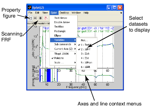
The graphical representation of the stack shown in figure 2.2 lets you do a number of manipulations witch are available trough the context menu of the list of datasets in the stack
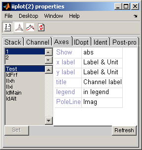
iiplot lets you display multiple axes see iicom Sub. Information about each axis is show in the axes tab.
For example open the interface with the commands below and see a few thing you can do
 ci=idcom;iicom(ci,'CurveLoad sdt_id');
 ci.Stack{'IdFrf'}=ci.Stack{'Test'}; % copy dataset
 ci.Stack{'IdFrf'}.xf=ci.Stack{'Test'}.xf*2; % double amplitude
 iicom('CurTab Axes');
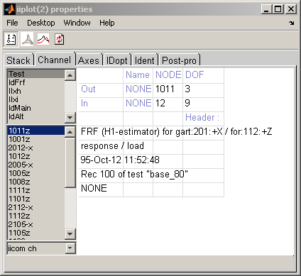
Once you have selected the datasets to be displayed, you can use the channel tab to scan trough the data.
Major commands you might want to know

 to scan trough different transfer functions. Note that you can also use the + or - keys when a drawing axis is active.
There are two main mechanisms to import FRF data into SDT. Universal files are easiest if generated by your acquisition system. Writing of an import script defining fields used by SDT is also fairly simple and described below (you can then use ufwrite to generate universal files for export).
The ufread and ufwrite functions allow conversions between the xf format and files in the Universal File Format which is supported by most measurement systems. A typical call would be
 fname=demosdt('build gartid.unv'); % generate the gartid.unv file
 UFS=ufread(fname);                 % read
 ci=idcom;   % For identification purposes open IDCOM
 ci.Stack{'curve','Test'}=UFS(1);  % Define FRFs in set 'Test'
 % possibly extract channels 1:4
 %  ci.Stack{'curve','Test'}=fe_def('SubDofInd',UFS(1),1:4)

 % To only view data in figure(11) the following would be sufficient
 cj=iiplot(11);      % open an iiplot in figure 11
 iiplot(cj,UFS(1));  % show UFS(1) there
where you read the database wrapper UFS (see xfopt), initialize the idcom figure, assign dataset 3 of UFS to dataset 'Test' 1 of ci (assuming that dataset three represents frequency response functions of interest).
Note that some acquisition systems write many universal files for a set of measurements (one file per channel). This is supported by ufread with a stared file name
UFS=ufread('FileRoot*.unv');
Measured frequency responses are stored in the .xf field (frequencies in .w) and should comply with the specifications of the xf format (see details under xf ). Other fields needed to specify the physical meaning of each FRF are detailed in the xfopt reference section. When importing data from your own format or using a universal file where some fields are not correct, the SDT will generally function with default values set by the xfopt function, but you should still complete/correct these variables as detailed below.
For correct display in feplot and title/legend generation, you should set the ci.Stack{'Test'}.dof field (see section 2.2 for details on geometry declaration, and mdof reference). For example one can consider a MIMO test with 2 inputs and 4 outputs stored as columns of field .xf with the rows corresponding to frequencies stored in field .w. You script will look like
 ci=idcom;
 [XF1,cf]=demosdt('demo2bay xf');% sample data and feplot pointer
 out_dof=[3:6]+.02'; % output dofs for 4 sensors in y direction
 in_dof=[6.02 3.01]; % input dofs for two shakers at nodes 1 and 10
 out_dof=out_dof(:)*ones(1,length(in_dof));
 in_dof=ones(length(out_dof),1)*in_dof(:)';
 XF1=struct('w',XF1.w, ...   % frequencies in Hz
            'xf',XF1.xf, ... % responses (size Nw x (40))
            'dof',[out_dof(:) in_dof(:)]);
 ci.Stack{'Test'}=XF1;          % sets data and verifies
 ci.IDopt.nsna=size(out_dof,1); % define IDCOM prop
 ci.IDopt.recip='mimo';         % define IDCOM prop
 iicom(ci,'sub');

 cf.def=ci.Stack{'Test'}; fecom('ch35'); % frequency of first mode
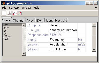
You can also edit these values using the iiplot properties:channel tab.
For correct identification using id_rc, you should verify the fields of ci.IDopt. These correspond to the IDcomGUI:Options tab (see section 2.3). You can also edit these values in a script. For correct identification, you should set
 ci=demosdt('demogartid');
 ci.IDopt.Residual='3';
 ci.IDopt.DataType='Acc';
 ci.IDopt.Absci='Hz';
 ci.IDopt.PoleU='Hz';
 iicom('wmin 6 40') % sets ci.IDopt.Selected
 ci.IDopt.Fit='Complex';
 ci.IDopt  % display current options
For correct transformations using id_rm, you should also verify ci.IDopt.NSNA (number of sensors/actuators), ci.IDopt.Reciprocity and ci.IDopt.Collocated.
For correct labels using iiplot you should set the abscissa, and ordinate numerator/denominator types in the data base wrapper. You can edit these values using the iiplot properties:channel tab. A typical script would declare frequencies, acceleration, and force using (see list with xfopt _datatype)
UFS(2).x='Freq';UFS(2).yn='Acc';UFS(2).yd='Load';UFS(2).info
ci=iicom('curveload gartid');
ci.Stack{'Test'}.yn.unit='N';
ci.Stack{'Test'}.yd.unit='M';
iicom sub
With SDT 6, global variables are no longer used and iiplot supports display of curves in other settings than identification.
If you have saved SDT 5 datasets into a .mat file, iicom('CurveLoad FileName') will place the data into an SDT 6 stack properly. Otherwise for an operation similar to that of SDT 5, where you use XF(1).xf rather than the new ci.Stack{'Test'}.xf, you should start iiplot in its identification mode and obtain a pointer XF (SDT handle object) to the data sets (now stored in the figure itself) as follows
 >> ci=iicom('curveid');XF=iicom(ci,'curveXF')

XF (curve stack in figure 2) =

XF(1) : [.w    0x0, xf    0x0] 'Test'  : response (general or unknown)
XF(2) : [.w    0x0, xf    0x0] 'IdFrf'  : response (general or unknown)
XF(3) : [.w    0x0, xf    0x0] 'IIxh'  : response (general or unknown)
XF(4) : [.w    0x0, xf    0x0] 'IIxi'  : response (general or unknown)
XF(5) : [.po   0x0, res   0x0] 'IdMain'  : shape data
XF(6) : [.po   0x0, res   0x0] 'IdAlt'  : shape data
The following table lists the global variables that were used in SDT 5 and the new procedure to access those fields which should be defined directly.
| XFdof | described DOFs at which the responses/shapes are defined, see .dof field for response and shape data in the xfopt section, was a global variable pointed at by the ci.Stack{'name'}.dof fields. |
| IDopt | which contains options used by identification routines, see idopt) is now stored in ci.IDopt. |
| IIw | was a global variable pointed at by the ci.Stack{'name'}.w fields. |
| IIxf | (main data set) was a global variable pointed at by the ci.Stack{'Test'}.xf fields. |
| IIxe | (identified model) was a global variable pointed at by the ci.Stack{'IdFrf'}.xf fields. |
| IIxh | (alternate data set) was a global variable pointed at by the ci.Stack{'IIxh'}.xf fields. |
| IIxi | (alternate data set) was a global variable pointed at by the ci.Stack{'IIxi'}.xf fields. |
| IIpo | (main pole set) was a global variable pointed at by the ci.Stack{'IdMain'}.po fields. |
| IIres | (main residue set) was a global variable pointed at by the ci.Stack{'IdMain'}.res fields. |
| IIpo1 | (alternate pole set) was a global variable pointed at by the ci.Stack{'IdAlt'}.po fields. |
| IIres1 | (alternate residue set) was a global variable pointed at by the ci.Stack{'IdAlt'}.res fields. |
| XF |
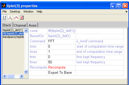
iiplot figure lets you perform standard signal processing operations (FFT, MMIF, filtering...) directly from the GUI. Opening iiplot properties figure, they are accessible trough the contextual menu compute (right click on the curve list in the Stack tab). Once an operation has been performed, its parameters can be edited in the GUI, and it can be recomputed using the Recompute button.
Following example illustrates some signal processing commands.
[mdl,def]=fe_time('demobar10-run'); % build mdl and perform time computation
cf=feplot(2); cf.model=mdl; cf.def=def;

ci=iiplot(3);
fecom(cf,'CursorOnIiplot') % display deformations in iiplot

% all following operations can be performed directly in the GUI:
% see the list of curves contained in iiplot figure, Stack tab:
iicom(ci,'pro');iicom(ci,'curtab Stack');
% compute FFT of deformations.  Name of entry 'feplot(2)_def(1)'
ename=ci.Stack(:,2); ename=ename{strncmp(ename,'feplot',5)};
ii_mmif('FFT',ci,ename) % compute
fname=sprintf('fft(%s)',ename);
iicom(ci,'curtab Stack',fname); % show FFT options that are editable
  % edit options & Recompute:
ci.Stack{fname}.Set={'fmax',50};
iicom(ci,'curtab Stack',fname,'Recompute');

% filter and display (the bandpass removes a lot of transient)
ii_mmif('BandPass -fmin 40 -fmax 50',ci,ename) % compute
fname=sprintf('bandpass(%s)',ename);
ci.Stack{fname}.Set={'fmin',10,'fmax',20};
iicom(ci,'curtab Stack',fname,'Recompute');
iicom(ci,'iix',{ename,fname});
This section lists various questions that were not answered elsewhere.
ci.ua.ob(1,11)=3; % define channel 3 as abscissa
iiplot;           % display the changes
set(ci.ga,'XLim',[0 1e-3]); % redefine axis bounds
%  sdtweb('demosdt.m#DemoGartteCurve') % FRF with 2 damping levels
ci=iiplot(demosdt('demogarttecurve'))
ci.Stack{'New'}
iicom(ci,'ChAllzeta')