PDF Index
|
Contents
Functions
PDF Index |
Identification is the process of estimating a parametric model (poles and modeshapes) that accurately represents measured data. The main algorithm proposed in the SDT is a frequency domain output error method that builds a model in the pole residue form (see section 5.6) through a tuning strategy. Key theoretical notions are pole/residue models, residual terms, and the relation between residues and modeshapes (see cpx).
Section 2.3.2 gives a tutorial on the standard procedure. Theoretical details about the underlying algorithm are given in section 2.3.3. Section 2.3.4 addresses its typical shortcomings. Other methods implemented in the SDT but not considered as efficient are addressed in later sections.
For the handling of MIMO tests, reciprocity,... see section 2.4. The gartid script gives real data and an identification result for the GARTEUR example. The demo_id script analyses a simple identification example.
For identification, the idcom interface uses a standard set of curves and identification options accessible from the IDopt tab or from the command line trough the pointer ci.IDopt. idcom(ci) turns the environment on, idcom(ci,'Off') removes options but not datasets.
ci=iicom('Curveid'); ci.Stack

    'curve'    'Test'      [1x1 struct]
    'curve'    'IdFrf'     [1x1 struct]
    'curve'    'IdMain'    [1x1 struct]
    'curve'    'IdAlt'     [1x1 struct]
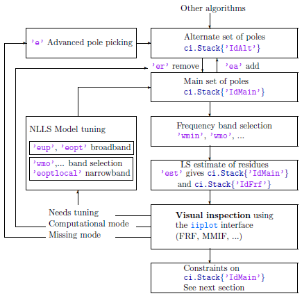
The id_rc identification method is based on an iterative refinement of the poles of the current model. Illustrated by the diagram below.
The main steps of the methodology are
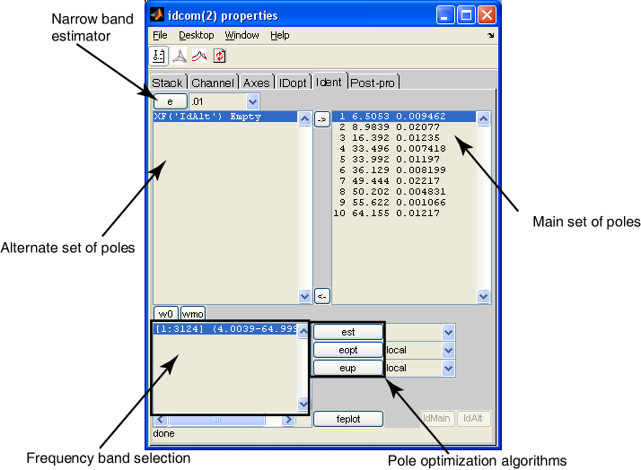
After verification of the Options tab of the idcom GUI figure, the Identification tab shown below gives you easy access to these steps (to open this figure, just run idcom from the MATLAB prompt). More details on how to proceed for each step are given below using data of the demo_id script.
The iteratively refined model is fully characterized by its poles (and the measured data). It is thus convenient to cut/paste the pole estimates into and out of a text editor (you can use the context menu of the main pole set to display this in the MATLAB command window). Saving the current pole set in a text file as the lines
 ci.Stack{'IdMain'}.po =[...
            1.1298e+02   1.0009e-02
            1.6974e+02   1.2615e-02
            2.3190e+02   8.9411e-03];
gives you all you need to recreate an identified model (even if you delete the current one) but also lets you refine the model by adding the line corresponding to a pole that you might have omitted. The context menu associated with the pole set listboxes lets you easily generate this list.
1 finding initial pole estimates, adding missed poles, removing computational poles
Getting an initial estimate of the poles of the model is the first difficulty. Dynamic responses of structures, typically show lightly damped resonances. The easiest way to build an initial estimate of the poles is thus to use a sequence of narrow band single pole estimations near peaks of the response or minima of the Multivariate Mode Indicator function (use iicom Showmmi and see ii_mmif for a full list of mode indicator functions).
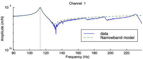
The idcom e command (based on a call to the ii_poest function) lets you to indicate a frequency (with the mouse or by giving a frequency value) and seeks a single pole narrow band model near this frequency (the pole is stored in ci.Stack{'IdAlt'}. Once the estimate found the iiplot drawing axes are updated to overlay ci.Stack{'Test'} and ci.Stack{'IdFrf'}.
In the plot shown above the fit is clearly quite good. This can also be judged by the information displayed by ii_poest
 LinLS:  1.563e-11, LogLS  8.974e-05, nw 10
 mean(relE) 0.00, scatter 0.00
 Found pole at 1.1299e+02   9.9994e-03
which indicates the linear and quadratic costs in the narrow frequency band used to find the pole, the number of points in the band, the mean relative error (norm of difference between test and model over norm of response which should be below 0.1), and the level of scatter (norm of real part over norm of residues, which should be small if the structure is close to having modal damping).
If you have a good fit and the pole differs from poles already in you current model, you can add the estimated pole (add poles in ci.Stack{'IdAlt'} to those in ci.Stack{'IdMain'}) using the idcom ea command (or the associated button). If the fit is not appropriate you can change the number of selected points/bandwidth and/or the central frequency. In rare cases where the local pole estimate does not give appropriate results you can add a pole by just indicating its frequency (f command) or you can use the polynomial (id_poly), direct system parameter (id_dspi), or any other identification algorithm to find your poles. You can also consider the idcom find command which uses the MMIF to seek poles that are present in your data but not in ci.Stack{'IdMain'}.
In cases where you have added too many poles to your current model, the idcom er command then lets you remove certain poles.
This phase of the identification relies heavily on user involvement. You are expected to visualize the different FRFs (use the +/- buttons/keys), check different frequency bands (zoom with the mouse and use iicom w commands), use Bode, Nyquist, MMIF, etc. (see iicom Show commands). The iiplot graphical user interface was designed to help you in this process and you should learn how to use it (you can get started in section 2.1).
2 estimating residues and residual terms
Once a model is created (you have estimated a set of poles), idcom est determines residues and displays the synthesized FRFs stored in ci.Stack{'IdFrf'}. A careful visualization of the data often leads to the discovery that some poles are missing from the initial model. The idcom e and ea commands can again be used to find initial estimates for the missing poles.
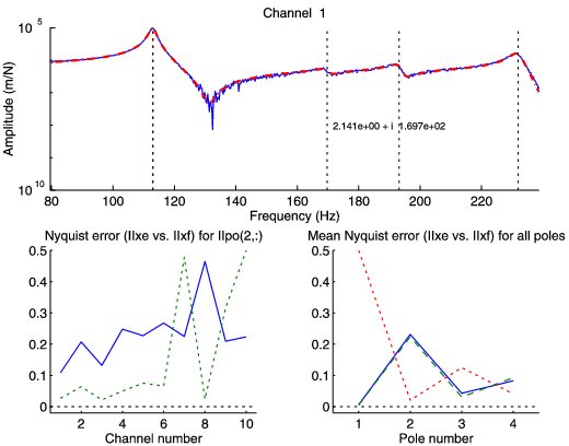
The need to add/remove poles is determined by careful examination of the match between the test data ci.Stack{'Test'} and identified model ci.Stack{'IdFrf'}. You should take the time to scan through different sensors, look at amplitude, phase, Nyquist, ...
Quality and error plots are of particular interest. The quality plot (lower right, obtained with iicom Showqual) gives an indication of the quality of the fit near each pole. Here pole 2 does not have a very good fit (relative error close to 0.2)but the response level (dotted line) is very small. The error plot (lower left, obtained with iicom Showerr) shows the same information for the current pole and each transfer function (you change the current pole by clicking on pole lines in the top plot). Here it confirms that the relative Nyquist error is close to 0.2 for most channels. This clearly indicates the need to update this pole as detailed in the next section (in this example, the relative Nyquist error is close to 0.1 after updating).
3 updating poles of the current model using a broad or narrow frequency band update
The various procedures used to build the initial pole set (see step 1 above) tend to give good but not perfect approximations of the pole sets. In particular, they tend to optimize the model for a cost that differs from the broadband quadratic cost that is really of interest here and thus result in biased pole estimates.
It is therefore highly desirable to perform non-linear update of the poles in ci.Stack{'IdMain'}. This update, which corresponds to a Non-Linear Least-Squares minimization, can be performed using the commands idcom eup (id_rc function) and eopt (id_rcopt function). The optimization problem is very non linear and non convex, good results are thus only found when improving results that are already acceptable (the result of phase 2 looks similar to the measured transfer function).
When using the eup command id_rc starts by reminding you of the currently selected options (accessible from the figure pointer ci.IDopt) for the type of residual corrections, model selected and, when needed, partial frequency range selected
 Low and high frequency mode correction
 Complex residue symmetric pole pattern
the algorithm then does a first estimation of residues and step directions and outputs
  %  mode#   dstep (%)     zeta      fstep (%)     freq
       1      10.000    1.0001e-02    -0.200    7.1043e+02
       2     -10.000    1.0001e-02     0.200    1.0569e+03
       3      10.000    1.0001e-02    -0.200    1.2176e+03
       4      10.000    1.0001e-02    -0.200    1.4587e+03
 Quadratic cost
    4.6869e-09
 Log-mag least-squares cost
    6.5772e+01
 how many more iterations? ([cr] for 1, 0 to exit) 30
which indicates the current pole positions, frequency and damping steps, as well as quadratic and logLS costs for the complete set of FRFs. These indications and particularly the way they improve after a few iterations should be used to determine when to stop iterating.
Here is a typical result after about 20 iterations
  %  mode#   dstep (%)     zeta      fstep (%)    freq
       1      -0.001    1.0005e-02     0.000    7.0993e+02
       2      -0.156    1.0481e-02    -0.001    1.0624e+03
       3      -0.020    9.9943e-03     0.000    1.2140e+03
       4      -0.039    1.0058e-02    -0.001    1.4560e+03
 Quadratic cost
  4.6869e-09 7.2729e-10 7.2741e-10 7.2686e-10 7.2697e-10
 Log-mag least-squares cost
  6.5772e+01 3.8229e+01 3.8270e+01 3.8232e+01 3.8196e+01
how many more iterations? ([cr] for 1, 0 to exit) 0
Satisfactory convergence can be judged by the convergence of the quadratic and logLS cost function values and the diminution of step sizes on the frequencies and damping ratios. In the example, the damping and frequency step-sizes of all the poles have been reduced by a factor higher than 50 to levels that are extremely low. Furthermore, both the quadratic and logLS costs have been significantly reduced (the leftmost value is the initial cost, the right most the current) and are now decreasing very slowly. These different factors indicate a good convergence and the model can be accepted (even though it is not exactly optimal).
The step size is divided by 2 every time the sign of the cost gradient changes (which generally corresponds passing over the optimal value). Thus, you need to have all (or at least most) steps divided by 8 for an acceptable convergence. Upon exit from id_rc, the idcom eup command displays an overlay of the measured data ci.Stack{'Test'} and the model with updated poles ci.Stack{'IdFrf'}. As indicated before, you should use the error and quality plots to see if mode tuning is needed.
The optimization is performed in the selected frequency range (idopt wmin and wmax indices). It is often useful to select a narrow frequency band that contains a few poles and update these poles. When doing so, model poles whose frequency are not within the selected band should be kept but not updated (use the euplocal and eoptlocal commands). You can also update selected poles using the 'eup num i' command (for example if you just added a pole that was previously missing).
id_rc (eup command) uses an ad-hoc optimization algorithm, that is not guaranteed to improve the result but has been found to be efficient during years of practice. id_rcopt (eopt command) uses a conjugate gradient algorithm which is guaranteed to improve the result but tends to get stuck at non optimal locations. You should use the eopt command when optimizing just one or two poles (for example using eoptlocal or 'eopt num i' to optimize different poles sequentially).
In many practical applications the results obtained after this first set of iterations are incomplete. Quite often local poles will have been omitted and should now be appended to the current set of poles (going back to step 1). Furthermore some poles may be diverging (damping and/or frequency step not converging towards zero). This divergence will occur if you add too many poles (and these poles should be deleted) and may occur in cases with very closely spaced or local modes where the initial step or the errors linked to other poles change the local optimum for the pole significantly (in this case you should reset the pole to its initial value and restart the optimization).
Once a good complex residue model obtained, one often seeks models that verify other properties of minimality, reciprocity or represented in the second order mass, damping, stiffness form. These approximations are provided using the id_rm and id_nor algorithms as detailed in section 2.4.
The id_rc algorithm (see [7][8]) seeks a non linear least squares approximation of the measured data
| p model = argmin |
| ⎛ ⎝ | αjk( id)(ωl,p)−αjk( test)(ωl) | ⎞ ⎠ | 2 (2.1) |
for models in the nominal pole/residue form (also often called partial fraction expansion [9])
| [α(s)] = |
| ⎛ ⎜ ⎜ ⎝ |
| + |
| ⎞ ⎟ ⎟ ⎠ | + [E] + |
| = [Φ(λj,s)][Rj,E,F] (2.2) |
or its variants detailed under res .
These models are linear functions of the residues and residual terms [Rj,E,F] and non linear functions of the poles λj. The algorithm thus works in two stages with residues found as solution of a linear least-square problem and poles found through a non linear optimization.
The id_rc function (idcom eup command) uses an ad-hoc optimization where all poles are optimized simultaneously and steps and directions are found using gradient information. This algorithm is usually the most efficient when optimizing more than two poles simultaneously, but is not guaranteed to converge or even to improve the result.
The id_rcopt function (idcom eopt command) uses a gradient or conjugate gradient optimization. It is guaranteed to improve the result but tends to be very slow when optimizing poles that are not closely spaced (this is due to the fact that the optimization problem is non convex and poorly conditioned). The standard procedure for the use of these algorithms is described in section 2.3.2. Improved and more robust optimization strategies are still considered and will eventually find their way into the SDT.
This section gives a few examples of cases where a direct use of id_rc gave poor results. The proposed solutions may give you hints on what to look for if you encounter a particular problem.
In many cases frequencies of estimated FRFs go down to zero. The first few points in these estimates generally show very large errors which can be attributed to both signal processing errors and sensor limitations. The figure above, shows a typical case where the first few points are in error by orders of magnitude. Of two models with the same poles, the one that keeps the low frequency erroneous points (- — -) has a very large error while a model truncating the low frequency range (- - -) gives an extremely accurate fit of the data (—).
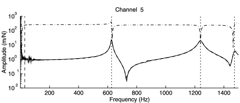
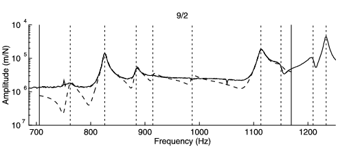
The fact that appropriate residual terms are needed to obtain good results can have significant effects. The figure above shows a typical problem where the identification is performed in the band indicated by the two vertical solid lines. When using the 7 poles of the band, two modes above the selected band have a strong contribution so that the fit (- - -) is poor and shows peaks that are more apparent than needed (in the 900-1100 Hz range the FRF should look flat). When the two modes just above the band are introduced, the fit becomes almost perfect (- — -) (only visible near 750 Hz).
Keeping out of band modes when doing narrow band pole updates is thus quite important. You may also consider identifying groups of modes by doing sequential identifications for segments of your test frequency band [8].
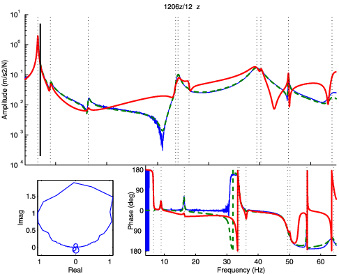
The example below shows a related effect. A very significant improvement is obtained when doing the estimation while removing the first peak from the band. In this case the problem is actually linked to measurement noise on this first peak (the Nyquist plot shown in the lower left corner is far from the theoretical circle).
Other problems are linked to poor test results. Typical sources of difficulties are
A class of identification algorithms makes a direct use of the second order parameterization. Although the general methodology introduced in previous sections was shown to be more efficient in general, the use of such algorithms may still be interesting for first-cut analyses. A major drawback of second order algorithms is that they fail to consider residual terms.
The algorithm proposed in id_dspi is derived from the direct system parameter identification algorithm introduced in Ref. [10]. Constraining the model to have the second-order form
| (2.3) |
it clearly appears that for known [cT], {yT}, {uT} the system matrices [CT], [KT], and [bT] can be found as solutions of a linear least-squares problem.
For a given output frequency response {yT}=xout and input frequency content {uT}=xin, id_dspi determines an optimal output shape matrix [cT] and solves the least squares problem for [CT], [KT], and [bT]. The results are given as a state-space model of the form
| (2.4) |
The frequency content of the input {u} has a strong influence on the results obtained with id_dspi. Quite often it is efficient to use it as a weighting, rather than using a white input (column of ones) in which case the columns of {y} are the transfer functions.
As no conditions are imposed on the reciprocity (symmetry) of the system matrices [CT] and [KT] and input/output shape matrices, the results of the algorithm are not directly related to the normal mode models identified by the general method. Results obtained by this method are thus not directly applicable to the prediction problems treated in section 2.4.2.
Among other parameterizations used for identification purposes, polynomial representations of transfer functions (5.27) have been investigated in more detail. However for structures with a number of lightly damped poles, numerical conditioning is often a problem. These problems are less acute when using orthogonal polynomials as proposed in Ref. [11]. This orthogonal polynomial method is implemented in id_poly, which is meant as a flexible tool for initial analyses of frequency response functions. This function is available as idcom poly command.