feutilb, fe

Contents Functions

feutilb, fe_caseg

Purpose

Gateway functions for advanced FEM utilities in SDT.

Description

This function is only used for internal SDT operation and actual implementation will vary over time. The following commands are documented to allow user calls and SDT source code understanding.

Assemble

Optimized strategies for assembly are provided in SDT through the Assemble command. More details are given in section 4.5.8.

AddNode

This command provides optimized operation when compared to the feutil equivalent and finer control.

CombineModel

mo1=feutilb('combinemodel',mo1,mo2);
[mo1,r1]=feutilb('combinemodel',mo1,mo2);

Integrated combining of two separate models. This call aims at creating an assembly from two separate mechanical components. This command properly handles potential NodeId, EltId, ProId, or MatId ovelaying by setting disjoint ID sets before assembly. Stack or Case entries with overlaying names are resolved, adding (1) to common names in the second model. Sets with identical names between both models are contatenated into a single set. The original numbering matrix for mo2 is output as a second argument (r1 in the second exemple call).

mo1 is taken as the reference to which mo2 will be added, the Node/Elt appending is performed by feutilAddTest.

Command option -cleanMP cleans up duplicated mat/pro entries in the combined model.
Command option -noSetCat, forces the sets duplication with incremented names (adding (1)), instead of concatenation when sets with identical names are found.
Command option CompatNodeElt asks not to shift NodeId and EltId in the second model. It then assumes the ID ranges are fully compatible in both models.
Command option CompatMatPro asks not to shift MatId and ProId in the second model. It then assumes these IDs to be fully compatible between both models.
Command option CompatBas asks no to shift the BasId in the second model. It then assumes these IDs to be fully compatible between both models.

dTKT

K = feutilb('dtkt',T,K) functional equivalent to diag(T'*k*T) but this call supports out of core and other optimized operations obtained through compiled functionalities. K may be a cell array of matrices, in which case one operates on each cell of the array.

GeomRB, ...

def=feutilb('geomrb',node,RefXYZ,adof,m) returns a geometric rigid body modes. If a mass matrix consistent with adof is provided the total mass, position of the center of gravity and inertia matrix at CG is computed. You can use def=feutilb('geomrb cg',Up) to force computation of rigid body mass properties.

def=feutilb('geomrbMass',model) returns the rigid body modes and mass, center of gravity and inertia matrix information.

il=feutilb('GeomRBBeam1',mdl,RefXYZ) returns standard p_beam properties for a given model section where RefXYZ is the coordinates of the reference point from the gravity center.

Match

Non conform mesh matching utilities. The objective is to return matching elements and local coordinates for a list of nodes.

Matching elements mean

for volumes, that the physical node is within the element. If volumes may be negative, check orientation using feutil orient.
for surfaces, that that the orthogonal projection of the node is within the element
for lines that the orthogonal projection on the line is between the line extremities.

A typical node matching call would be

model=femesh('test hexa8');
match=struct('Node',[.1 .1 .1;.5 .5 .5;1 1 1]);
match=feutilb('match -info radius .9 tol 1e-8',model,match)

Accepted command options are

MatchSurf has the same objective but uses a completely different strategy to match nodes on a surface. This is typically well suited for contact applications.
radius rad. The search is limited to points that are not too far a way from matchable element centers. Defining a search radius manually can help prevent matching for elements that are too far away or on the contrary allow matching within elements that are very large so that interior points may be far from the center.
tolval modifies the 1e-8 tolerance used to stop the non-linear search for the match point in second order elements

The output structure contains the fields

.Node	original positions
.rstj	position in element coordinates and jacobian information.
.StickNode	orthogonal projection on element surface if the original node is not within the element, otherwise original position.
.Info	one row per matched node/element giving NodeId if exact match, number of nodes per element, and element type.
.match	obtained when calling the command with -info, typically for row by row post-processing of the match. A cell array with one row per matched node/element giving eltname, slave element row, rstj, sticknode

MpcFromMatch

This command is used to build multiple point constraints from a match.
feutilb('MpcFromMatch',model,match).

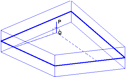
The solution retained for surfaces is to first project the arbitrarily located connection point P on the element surface onto a point Q on the neutral fiber used where element nodes are located. Then Q1 or P1 shape functions and their derivatives are used to define a linear relation between the 6 degree of freedom of point Q and the 3 or 4 nodes of the facing surface. Motion at P is then deduced using a linearized rigid PQ link. One chooses to ignore rotations at the nodes since their use is very dependent on the shell element formulation.

Figure 9.2: Non conform mesh handling

The local element coordinates are defined by x_j^e,j=1:3 along the r coordinate line

x_j^e = α_x

∂ N_i

∂ r

x_ij with α_x=1/

⎪⎪
⎪⎪
⎪⎪
⎪⎪

∂ N_i

∂ r

x_ij

⎪⎪
⎪⎪
⎪⎪
⎪⎪

(9.1)

y^e that is orthogonal to x^e and in the x^e, ∂ N_i/∂ sx_ij plane, and z^e that defines an orthonormal basis.

The local rotations at point Q are estimated from rotations at the corner nodes using

R_j = x_j^e

∂ N_i

∂ y^e

u_ikz_k^e − y_j^e

∂ N_i

∂ x^e

u_ikz_k^e +

z_j^e

⎛
⎜
⎜
⎝

∂ N_i

∂ x^e

u_ik y_k^e −

∂ N_i

∂ y^e

u_ik x_k^e

⎞
⎟
⎟
⎠

(9.2)

with u_ik the translation at element nodes and j=1:3, i=1:N_node, k=1:3. Displacement at Q is interpolated simply from shape functions, displacement at P is obtained by considering that the segment QP is rigid.

For volumes, displacement is interpolated using shape functions while rotations are obtained by averaging displacement gradients in orthogonal directions

theta_x

⎛
⎝

−N_y,z+Nz,y

⎞
⎠

/2 {u}

theta_y

⎛
⎝

N_x,z−Nz,x

⎞
⎠

/2 {u}

theta_w

⎛
⎝

−N_x,y+Ny,x

⎞
⎠

/2 {u}

(9.3)

You can check that the constraints generated do not constrain rigid body motion using fe_caseg('rbcheck',model) which builds the transformation associated to linear constraints and returns a list of DOFs where geometric rigid body modes do not coincide with the transformation.

PlaceInDof

def2 = feutilb('PlaceInDof',DOF,def) returns a structure with identical fields but with shapes ordered using the specified DOF. This is used to eliminate DOFs, add zeros for unused DOFs or simply reorder DOFs. See also fe_def SubDof.

StressCut

The StressCut command is the gateway for dynamic stress observation commands. Typicall steps of this command are

View mesh generation, see section 4.4.1.
Generate a selection sel=fe_caseg('stresscut -selout',VIEW,model);
Display the selection in feplot using fe_caseg('stresscut',sel,cf)
Observe the result using curve=fe_caseg('StressObserve',cf.sel(2),def)

For the selection generation, accepted options are

VIEW can be a mesh so that feutilb Match is used find elements associated with viewing positions. A structure struct('type','Gauss') to return selection at Gauss points. A structure struct('type','BeamGauss') to return selection at beam Gauss points.
a model or feplot handle cf can be provided as third argument.
-SelOut requires selection output.
-Radiusval provides a search radius for the feutilb Match call.

The sel data structure is a standard selection (see feplot sel) with additional field .StressObs a structure with the following fields

.cta observation matrix for stress components. The expected sort is to have all components at first node, all at second node, ...
.DOF expected DOF needed for the observation.
.X,.Xlab labels for the observation, see Multi-dim curve for details.
.CritFcn callback to be evaluated, see fe_stress CritFcn.
.Node,.Elt nodes and elements for the view mesh.
.trans structure for the observation of interpolated displacement (needed when view mesh nodes are not nodes of the original mesh).

StressObserve

The StressCut command typically returns all stress components (x, y, and z), for a relevant plot, it is useful to define a further post-treatment, using the sel.StressObs.CritFcn callback. This callback is called once the stress observation have been performed. The current result is stored in variable r1, and follows the dimensions declared in field .X of the observation. For example to extract stresses in the x direction, the callback is

 sel.StressObs.CritFcn='r1=r1(1,:,:);';

The StressObserve command outputs the stress observation in an curve structure. You can provide a callback -crit "my_callback". If empty, all components are kept.

data=fe_caseg('StressObserve -crit""',cf.sel(2),def);
iiplot(data); % plot results

TKT

K = feutilb('tkt',T,K) functional equivalent to T'*k*T but this call supports out of core and other optimized operations obtained through compiled functionalities. K may be a cell array of matrices, in which case one operates on each cell of the array.

Write

feutilb('WriteFileName.m',model) writes a clean output of a model to a script. Without a file name, the script is shown in the command window.

feutilb('_writeil',model) writes properties. feutilb('_writepl',model) writes materials.

ZoomClip

The command accessible through the axes context menu Clip, can now also be called from the command line fe_caseg('ZoomClip',cf.ga,[xyz_left;xyz_right]).