2.4 Using shaped orthotropic piezoelectric transducers
2.4.1 Introduction
Typical piezoelectric transducers found on the market are rectangular or circular. Different researchers have however studied the possibility to use more complex shapes. This idea was mainly driven by the active control applications. The first developments in this direction concern triangular actuators which will be used in the following example after recalling the theory behind the development of such transducers. When used as an actuator, an applied voltage on a piezoelectric patch results in a set of balanced forces on the supporting structure. The analytical expression of these so-called equivalent forces has been derived analytically in [] in the general case of an orthotropic patch poled through the thickness with an arbitrary shape and attached to a supporting plate (assumed to follow Kirchhoff plate theory). The analytical expressions show that these forces are a function of the material properties of the piezo, as well as the expression of the normal to the contour of the patch. In the case of a triangular patch, the equivalent forces are illustrated on Figure 2.28. They consist in point forces P and P/2, and bending moments M1 and M2 whose expressions are:
These expressions show that the point forces are only present when the material is orthotropic (e31 ≠ e32). An interesting application of the triangular actuator is to design it to be a point-force actuator. This requires (i) to clamp the base of the triangle in order to cancel the bending moment M1 and the two point forces P/2, (ii) to cancel M2. The result is a single point-force P at the tip of the triangle. The cancelation of M2 requires to have []:
This expression shows that the point-force actuator can only be achieved when e31 and e32 are of opposite sign. With a PZT ceramic, this is possible using inter-digitated electrodes, which result in a compression in the lateral direction when the transducers elongates in the longitudinal direction. A possibility is to use a triangular transducer based on the same principle as the P1−type MFC. The resulting force at the tip of the triangle is given by:
| Figure 2.28: Equivalent loads for an orthotropic piezoelectric actuator |
Given the material properties of the active layer of P1-MFCs in Table 2.4, the values of e31 and e32 are:
and the b/l ratio leading to a point load actuator is
Another possibility is to use a full piezoceramic instead of a composite, which is illustrated below.
2.4.2 Example of a triangular point load actuator
We consider an example similar to the one treated in [] which consists in a 414mmx314mmx1mm aluminum plate clamped on its edges, on which a triangular piezoelectric transducer is fixed on the top surface in order to produce a point load, as illustrated in Figure 2.29. The piezoelectric material used is SONOX P502 whose properties are given in Table 1.2 with the exception that the value of νp=0.4 in order to be in accordance with the value used in []. With these material properties, the b/l ratio to obtain a point load actuator is b/l=0.336 (this will be verified in the example script). The triangular ceramic has a thickness of 180µ m and is encapsulated between two layers of epoxy (see properties in Table 2.2) which have a thickness of 60 µ m. The basis of the triangle is 33.6 mm in order to obtain the point load actuator (the height has a length of 100 mm). One triangle is attached to the top surface, and one to the bottom, and the transducers are driven out of phase in order to induce pure bending of the plate and no in-plane motion.
| Figure 2.29: Description of the numerical case study for a point load actuator |
2.4.3 Numerical implementation of the triangular point load actuator
The mesh used for the computations is shown in Figure 2.30 and is generated with:
( d_piezo('TutoPlate_triang-s1')
)
d_piezo('TutoPlate_triang-s1')
)
model=d_piezo('MeshTrianglePlate');
Note that because of the specific geometry of the surfaces including a triangle, it is not possible to mesh it with SDT commands, so that an external call to the software GMSH is made using fe_gmsh commands.
cf=feplot(model); fecom('colordatapro'); fecom('view2')
| Figure 2.30: Mesh of the aluminum plate with a triangular piezoelectric actuator |
The static response due to an applied voltage on the piezo actuators is computed as follows:
(d_piezo('TutoPlate_triang-s2')
)
model=fe_case(model,'SensDof','Tip',7.03);
model=fe_case(model,'DofSet','V-Act',struct('def',[-1; 1],'DOF',[100001; 100002]+.21));
(d_piezo('TutoPlate_triang-s3')
)
d0=fe_simul('dfrf',stack_set(model,'info','Freq',0));
cf.def=d0; fecom('colordataz -alpha .8 -edgealpha .1')
fecom('scd -.03'); fecom('view3');
and represented on Figure 2.31.
| Figure 2.31: Static displacement due to voltage actuation on the triangular piezo |
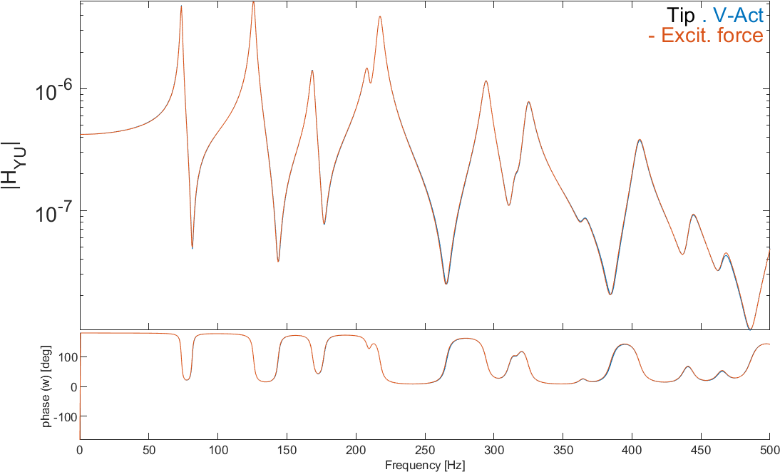
We now compute and compare the dynamic response of the plate excited with the triangular piezo and a point force whose amplitude is computed using Equation ((9)).
The computation is performed with a reduced state-space model using 20 mode shapes:
(d_piezo('TutoPlate_triang-s4')
)
[sys,TR]=fe2ss('free 5 20 0 -dterm',model);
C1=qbode(sys,linspace(0,500,1000)'*2*pi,'struct'); C1.name='.';
model=fe_case(model,'Remove','V-Act');
model=fe_case(model,'FixDof','Piezos',[100001;100002]);
CC=p_piezo('viewdd -struct',model);
a=100; b=33.58;
zm=0.650e-3; V=1; e31=CC.e(1); A=-(e31*zm*V*b)/a; A=A*2;
bl= 2*sqrt(-CC.e(2)/CC.e(1));
data=struct('DOF',[7.03],'def',A); data.lab=fe_curve('datatype',13);
model=fe_case(model,'DofLoad','PointLoad',data);
d1=fe_simul('dfrf',stack_set(model,'info','Freq',0));
ind=fe_c(d1.DOF,7.03,'ind'); d1p=d1.def(ind);
[sys,TR]=fe2ss('free 5 20 0 -dterm',model);
C2=qbode(sys,linspace(0,500,1000)'*2*pi,'struct'); C2.name='-';
ci=iiplot;
iicom(ci,'curveinit',{'curve',C1.name,C1;'curve',C2.name,C2});
iicom('submagpha');
The amplitude and phase of the vertical displacement at the tip of the triangle are represented for both cases in Figure 2.32, showing the excellent agreement.
| Figure 2.32: Dynamic response at the tip of the triangle due to (i) voltage actuation on the piezo and (ii) point force at the tip of the triangle |
©1991-2023 by SDTools