Vibration damping using a tuned resonant shunt circuit

SDT-piezo Contents Functions

2.5 Vibration damping using a tuned resonant shunt circuit

2.5.1 Introduction

The idea of damping a structure via a resonant shunt circuit is very similar to the mechanical tuned mass damper (TMD) concept. The mechanical TMD is replaced by a 'RL' shunt circuit which, together with the capacitance of the piezoelectric element to which it is attached, acts as a resonant 'RLC' circuit. By tuning the resonance frequency of this circuit to the open-circuit (OC) resonance frequency of the structure equipped with a piezoelectric transducer, one can achieve vibration reduction around the resonant peak of interest. The mechanism is based on the conversion of part of the mechanical energy to electrical energy which is then dissipated in the resistive component of the circuit.

The part of mechanical energy which is converted into electrical energy is given by the generalized electro-mechanical coupling coefficient α_i of the mode i of interest. In practice, this generalized coupling coefficient can be computed based on the open-circuit (OC) and short-circuit (SC) frequencies Ω_i and ω_i of the piezoelectric structure. Experimentally, these frequencies are usually obtained via the measurement of the impedance (V/I) or the capacitance (Q/V) of the piezoelectric structure, and one has:

(12)

Once α_i is known for the mode of interest, the values of R and L can be computed. Several rules exist to compute the optimal values of R and L []. We adopt here Yamada's tuning rules which are equivalent to Den Hartog's tuning rules for the mechanical TMD. The first rule aims at tuning the resonant circuit to the OC frequency Ω_i of the piezoelectric structure:

(13)

with

(14)

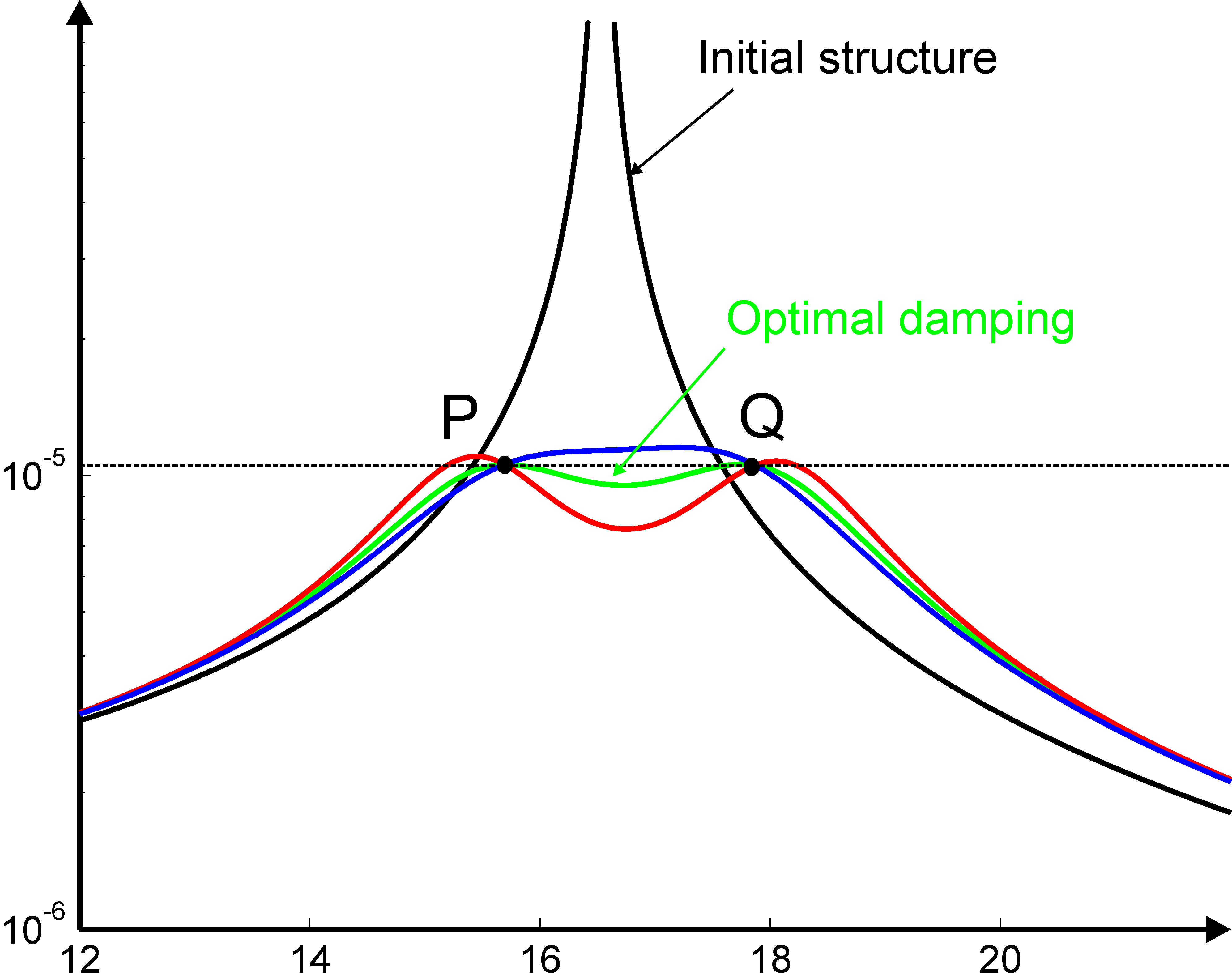
where C_i2 is the capacitance of the piezoelectric element attached to the structure taken after the resonant frequency of interest. Note that this value is in practice difficult to measure with precision. In this example, we will take the value which is at the frequency corresponding to the mean value between the SC resonant frequencies ω_i and ω_i+1. This first tuning rule allows to compute the value of L. For different values of R, one can show that when plotting the response of the structure to which the resonant shunt has been added for different values of R, all curves cross at two points P and Q which are at the same height (Figure 2.33). The second tuning rule is aimed at finding the optimal value of R which minimizes the response of the structure for the range of frequencies around the natural frequency of interest and is given by:

(15)

Figure 2.33: Response of the structure with and without and RL shunt : P and Q are at the same height when δ=1

2.5.2 Resonant shunt circuit applied to a cantilever beam

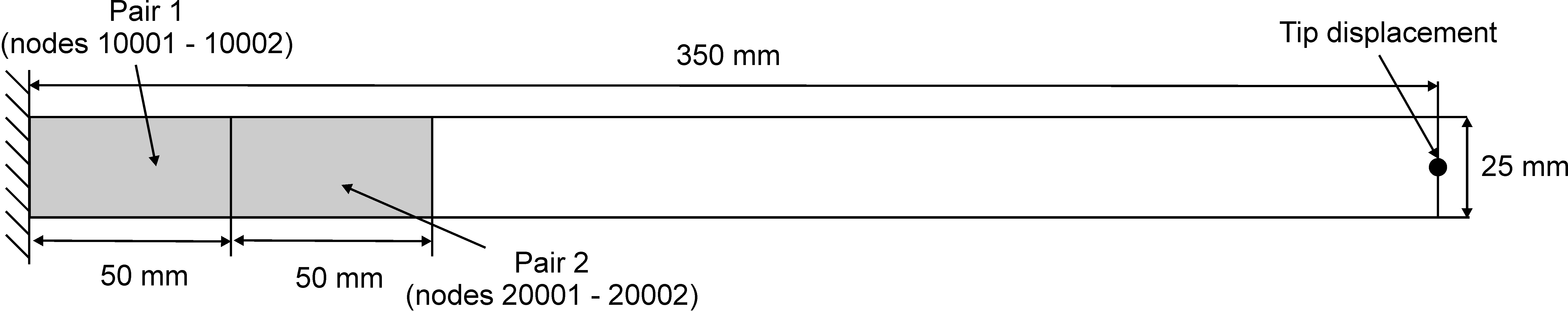
We illustrate the use of a resonant shunt with the following example of a cantilever beam. The beam is has a length of 350 mm, a width of 25 mm and a height of 2 mm (Figure 2.34). Two pairs of piezoelectric PIC 255 patches of dimensions 50 mm X 25 mm X 0.5 mm are glued on each side of the beam starting at the cantilever side . The nodes associated to the electrical dofs of the four patches are numbered respectively [10001 10002] for the patches next to the clamping side, and [20001 20002] for the other pair situated next to it.

Figure 2.34: Cantilever beam with two pairs of piezoelectric patches

Figure 2.35: Mesh of the cantilever beam showing the two pairs of piezoelectric patches on the left, next to the clamp

We start by generating the mesh (Figure 2.35) and setting the damping in the model.
(d_piezo('TutoPz_shunt-s1') )

% See full example as MATLAB code in d_piezo('ScriptTutoPz_Shunt')
%% Step 1 - Build mesh and visualize
% Meshing script can be viewed with sdtweb d_piezo('MeshShunt')
model=d_piezo('meshshunt');
model=stack_set(model,'info','DefaultZeta',1e-4);

feplot(model); cf=fecom; fecom('colordatapro')

In order to implement the shunt, we will compute the capacitance curve of the first set of patches used in phase opposition (bending) and extract the OC and SC first natural frequency of the cantilever beam. In order to do that, we define two combinations of patches for actuation (bending using the first pair in opposition of phase, and bending using the second pair in opposition of phase), one combination of charge sensors in opposition of phase (to compute the capacitance of the first pair), and one sensor for tip displacement (Figure 2.34).
(d_piezo('TutoPz_shunt-s2') )

%% Step 2 - Define actuators and sensors
% Actuators
data.def=[1 -1 0 0; 0 0 1 -1]'; % Define combinations for actuators
data.DOF=p_piezo('electrodedof.*',model); edof=data.DOF;
model=fe_case(model,'DofSet','Vin',data);
% Sensors
r1=struct('cta',[1 -1],'DOF',edof(1:2),'name','Qs');
model=p_piezo('ElectrodeSensQ',model,r1);
nd=feutil('find node x==350 & y==25',model);
model=fe_case(model,'SensDof','Tip',nd+.03);
sens=fe_case(model,'sens');

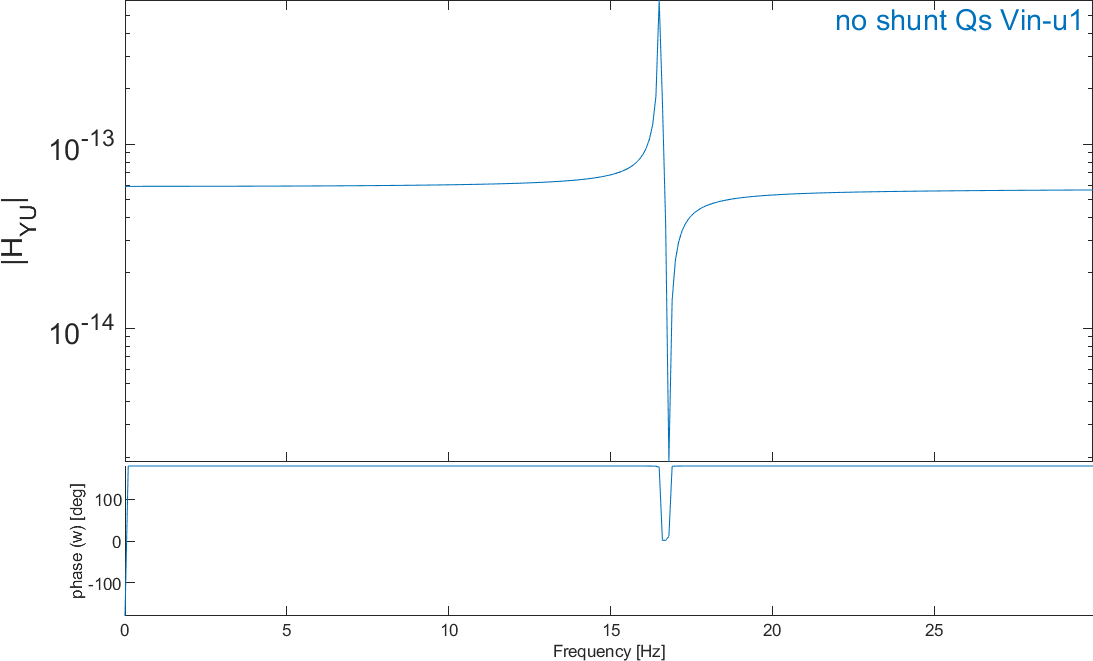
We can now compute the response of the structure to the two bending actuators using a reduced state-space model with 30 modes. The response of the combination of charge sensors is the capacitance curve (Figure 2.36) of the first pair of piezo patches used in opposition of phase from which ω₁ and Ω₁ are extracted to compute α₁, and C₁₂ is computed. Note that because the model is in millimiters, the voltage is expressed in µ V and the charge remains in Coulombs, so that the capacitance is expressed in MF (megaFarads) (see fe_mat ('convertSIMM') for details on the unit conversion when working in millimeters).

Figure 2.36: Capacitance (Q/V) of the first pair of piezo patches in bending. The resonance corresponds to ω₁ and the anti-resonance to Ω₁. C₁₂ is the capacitance in the flat part after the anti-resonance

 w=linspace(0,1e3,1e4)'*2*pi;
 [sys,TR]=fe2ss('free 5 30 0 -dterm',model);
 C1=qbode(sys,w,'struct'); C1.name='no shunt';

 ci=iiplot;
 iicom('CurveReset');iicom('curveinit',C1)
 iicom(ci,'xlim[0 30]') %

(d_piezo('TutoPz_shunt-s3') )

%% Step 3 - Determine parameters for shunt tuning
 % Extract w1 and W1 and compute alpha_1
C=C1.Y(:,1);
% Find poles and zeros of impedance (1/jwC)
if ~exist('findpeaks','file'); warning('Skipping step, signal toolbox');
return;end
[pksPoles,locsPoles]=findpeaks(abs(1./C)); Wi=w(locsPoles);
[pksZeros,locsZeros]=findpeaks(abs(C)); wi=w(locsZeros);
% concentrate on mode of interest (mode 1)
 W1=w(locsPoles(1)); w1=w(locsZeros(1));
% Compute alpha for mode of interest
a1=sqrt((W1^2-w1^2)/W1^2);

% Compute Cs2 for mode of interest
i1=1; i2=locsZeros(1); i3=locsZeros(2);
dw2=w(i3)-w(i2); wCs2=w(i2)+dw2/2;
[y,i]=min(abs(w-wCs2)); Cs2=abs(C(i));

We can now use Yamada's tuning rules to find R and L:

%% Determine shunt parameters (R and L) and apply it to damp 1st mode
% Tuning using Yamada's rule
d=1; r=sqrt((3*a1^2)/(2-a1^2));
L_Yam=1/d^2/Cs2/W1^2; R_Yam=r/Cs2/W1;

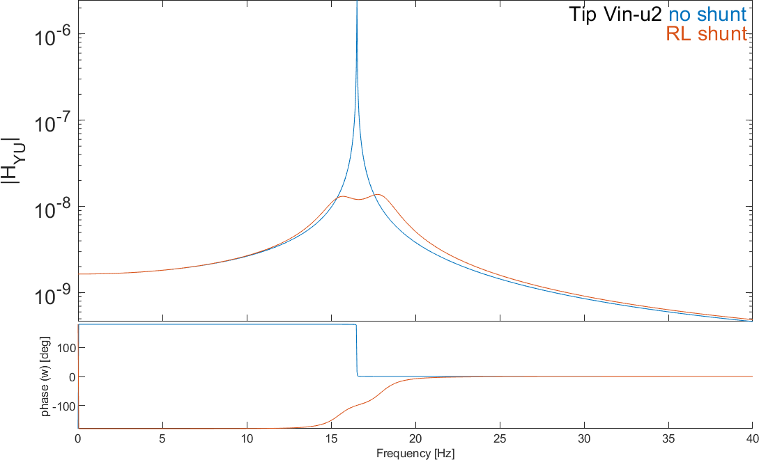
and represent the FRF of the tip displacement due to bending actuation on the second pair of piezos for the initial system and the system with the shunt (Figure 2.37). The shunt is implemented using the feedback function of the Control toolbox.
(d_piezo('TutoPz_shunt-s4') )

%% Step 4 - Compute dynamic response with optimal shunt
w=linspace(0,40,1e3)*2*pi;
C1=qbode(sys,w,'struct'); C1.name='no shunt';

% Implement shunt using feeback - requires control toolbox - compute FRF
if ~exist('feedback','file'); warning('Skipping step, control toolbox');
  return;
end
A=tf([L_Yam R_Yam 0],1); % RL shunt in tf form
sys2=feedback(sys,A,1,1,1);
% qbode does not work with feedback so use freqresp from control toolbox
 C=freqresp(sys2,w); a=C(:); C2=C1; C2.Y=reshape(a,4,1000)';
 C2.name='RL shunt';

% Plot and compare curves
iicom('CurveReset');
iicom(ci,'curveinit',{'curve',C1.name,C1;'curve',C2.name,C2});
iicom(ci,'ch 4')

Figure 2.37: Tip displacement due to the bending actuator of the second pair of piezo patches with and without shunt