 PDF Index
| SDT-piezo
Contents
Functions
PDF Index |
This application example deals with the determination of the sensitivity of a piezoelectric sensor to base excitation.
By far the most common sensor for measuring vibrations is the accelerometer. The basic working principle of such a device is presented in Figure 2.39(a). It consists of a moving mass on a spring and dashpot, attached to a moving solid. The acceleration of the moving solid results in a differential movement x between the mass M and the solid. The governing equation is given by,
| (16) |
In the frequency domain x/x0 is given by,
| (17) |
with ωn = √k/m and ξ=b/2√km and for frequencies ω << ωn, one has,
| (18) |
showing that at low frequencies compared to the natural frequency
of the mass-spring system, x is proportional to the acceleration
x0. Note that since the proportionality factor is
−1/ωn2, the sensitivity of the sensor is increased
as ωn2 is decreased. At the same time, the frequency band
in which the accelerometer response is proportional to
x0 is reduced.
(a) (b)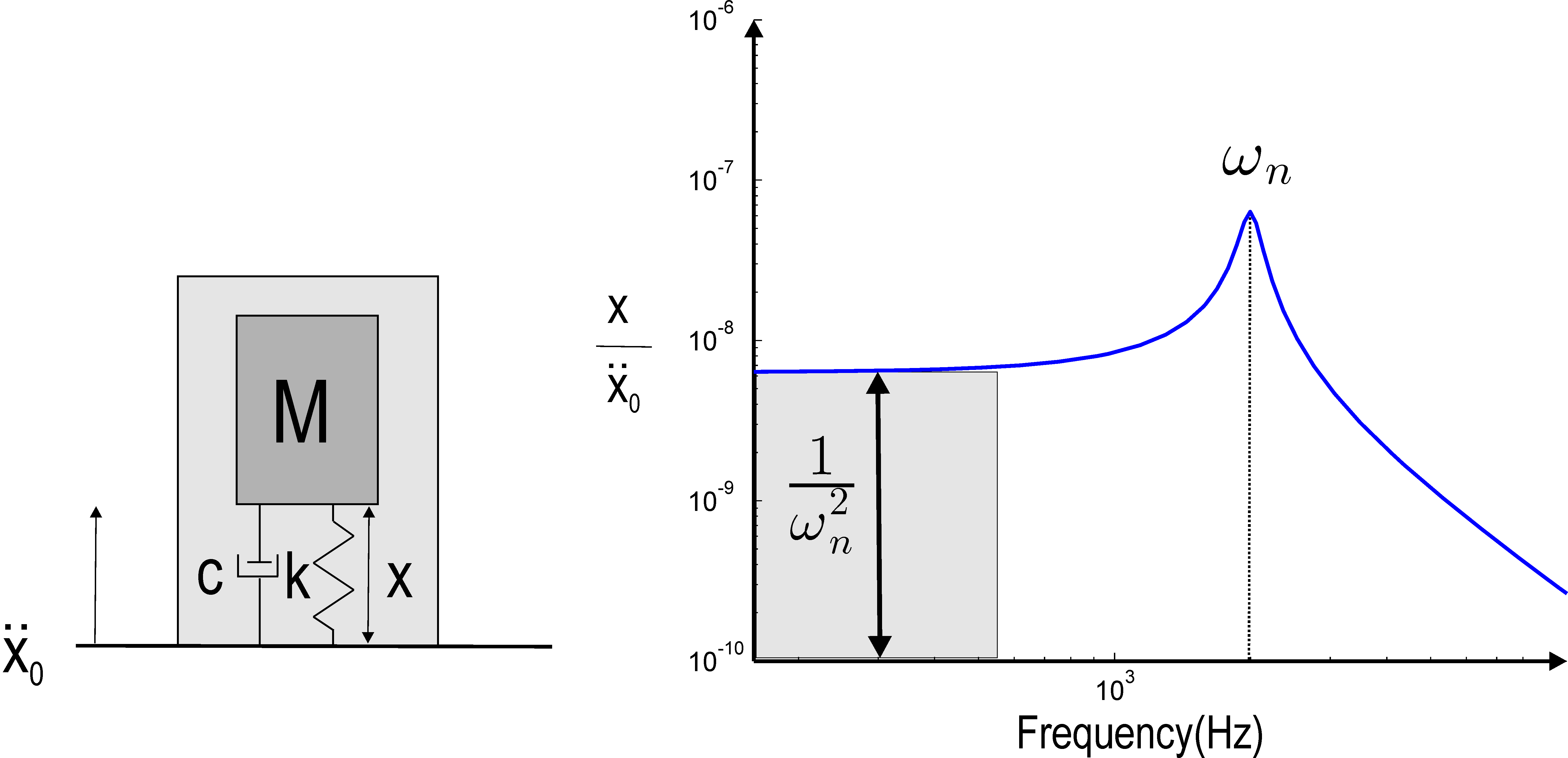
Figure 2.39: Working principle of an accelerometer
The relative displacement x can be measured in different ways
among which the use of piezoelectric material, either in longitudinal or shear mode (Figure 2.40).
In such configurations, the strain applied to the piezoelectric material is proportional to the relative displacement between the
mass and the base. If no amplifier is used, the voltage generated between the electrodes of the piezoelectric material is directly
proportional to the strain, and therefore to the relative displacement. For frequencies well below the natural frequency of
the accelerometer, the voltage produced is therefore proportional to the absolute acceleration of the base.
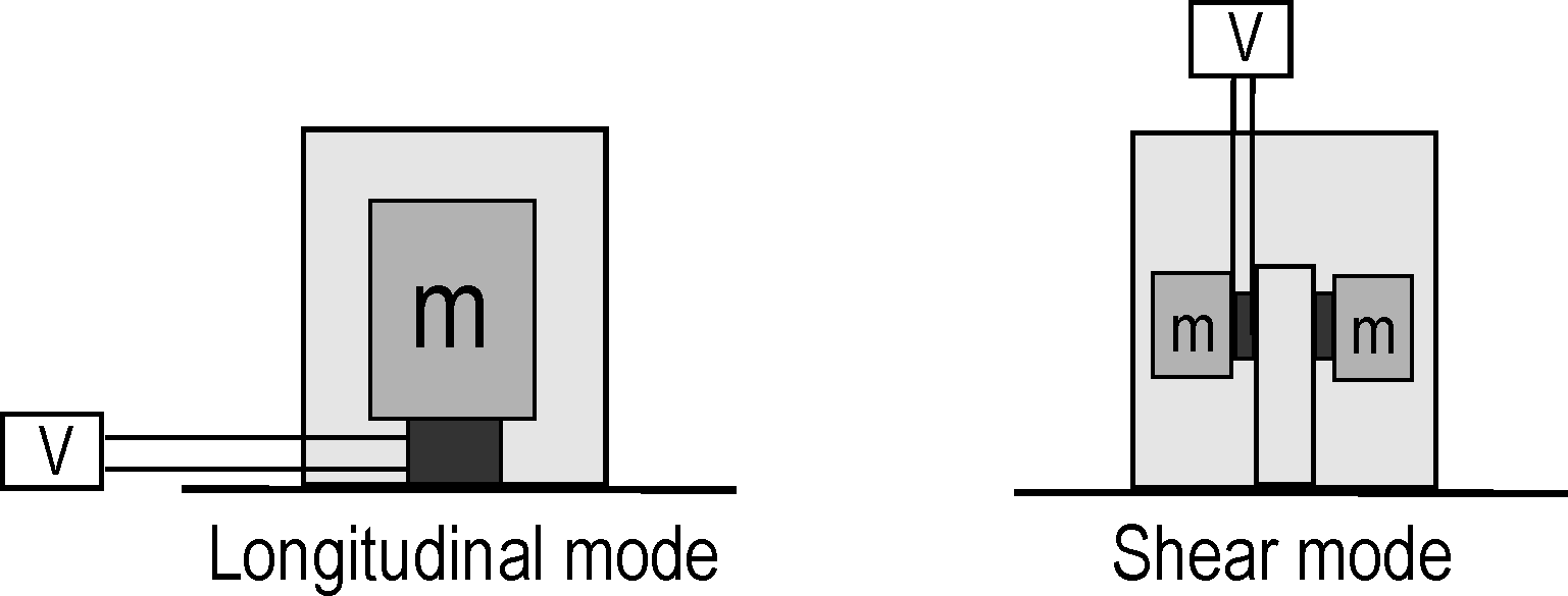
Figure 2.40: Different sensing principles for standard piezoelectric accelerometers
A basic design of a piezoelectric accelerometer working in the longitudinal mode is shown in Figure 2.38. In this example, the casing of the accelerometer is not taken into account, so that the device consists in a 3mm thick rigid wear plate (10mm diameter), a 1mm thick piezoelectric element (5mm diameter), and a 10mm thick (10mm diameter) steel proof mass. The mechanical properties of the three elements are given in Table 2.5. The piezoelectric properties of the sensing element are given in Table 2.6 and correspond to SONOX_P502_iso property in m_piezo Database. The sensing element is poled through the thickness and the two electrodes are on the top and bottom surfaces.
The sensitivity curve of the accelerometer, expressed in V/m/s2 is used to assess the response of the sensor to a base acceleration in the sensing direction (here vertical). In order to compute this sensitivity curve, one needs therefore to apply a uniform vertical base acceleration to the sensor and to compute the response of the sensing element as a function of the frequency.
This can be done in different ways. The following scripts compare two approaches. The first one consists in applying a uniform pressure on the base to excite the accelerometer. In this case, the pressure is constant, but the acceleration of the base is not strictly constant due to the flexibility of the wear plate. The second one consists in enforcing a constant vertical acceleration of all the nodes at the bottom of the base. In this case the acceleration is constant over the whole bottom surface of the accelerometer. The two approaches are compared in the following illustrative scripts.
( d_piezo('TutoAccel-s1')
)
d_piezo('TutoAccel-s1')
)
The mesh of the accelerometer is produced with the following call to d_piezo , see also a detailed description in Section 2.6. It is shown in Figure 2.41
% See full example as MATLAB code in d_piezo('ScriptTutoAccel')
%% Step 1 - Build Mesh and visualize
% Meshing script can be viewed with sdtweb d_piezo('MeshBaseAccel')
model=d_piezo('MeshBaseAccel');
cf=feplot(model); fecom('colordatagroup');
set(gca,'cameraposition',[-0.0604   -0.0787    0.0139])
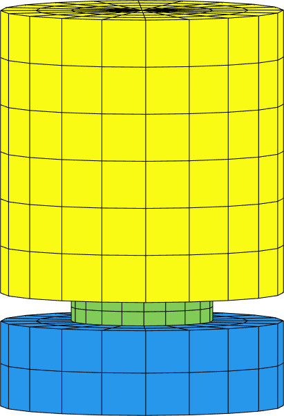
Figure 2.41: Mesh of the piezoelectric accelerometer. The different colors represent the different groups
The call includes the meshing of the accelerometer, the definition of material properties, as well as the definition of electrodes.
In addition, the bottom electrode is grounded, and both a voltage and a charge sensor are defined for the top electrode. A displacement sensor at the center of the base is defined in order to compute the sensitivity. The different calls used are:
(d_piezo('TutoAccel-s2')
)
%% Step 2 - Define sensors and actuators
% -MatID 2 requests a charge resultant sensor
% -vout requests a voltage sensor
model=p_piezo('ElectrodeMPC Top sensor -matid 2 -vout',model,'z==0.004');
% -ground generates a v=0 FixDof case entry
model=p_piezo('ElectrodeMPC Bottom sensor -ground',model,'z==0.003');
% Add a displacement sensor for the basis
model=fe_case(model,'SensDof','Base-displ',1.03);
The sensitivity for the sensor used in a voltage mode is then computed using the following script:
% Remove the charge sensor (not needed)
model=fe_case(model,'remove','Q-Top sensor');
% Normal surface force (pressure) applied to bottom of wear plate for excitation:
data=struct('sel','z==0','eltsel','groupall','def',1e4,'DOF',.19);
model=fe_case(model,'Fsurf','Bottom excitation',data);

% Other parameters
model=stack_set(model,'info','Freq',logspace(3,5.3,200)'); % freq. for computation
%% Step 3 - Compute dynamic response (full) and plot Bode diagram
ofact('silent'); d1=fe_simul('dfrf',model);

% Project on sensor
sens=fe_case(model,'sens');

% Build a clean "curve" for iiplot display
C1=fe_case('SensObserve -DimPos 2 3 1',sens,d1);C1.name='DFRF';C1.Ylab='Base-Exc';
C1.X{2}={'Sensor output(V)';'Base Acc(m/s^2)';'Sensitivity (V/m/s^2)'};
C1.Y(:,2)=C1.Y(:,2).*(-(C1.X{1}(:,1)*2*pi).^2); % Base acc =disp.*-w.^2
C1.Y(:,3)=C1.Y(:,1)./C1.Y(:,2);                 % Sensitivity=V/acc
C1=sdsetprop(C1,'PlotInfo','sub','magpha','scale','xlog;ylog');
C1.name='Free-Voltage';
ci=iiplot;
iicom(ci,'curveInit',C1.name,C1);iicom ch3; iicom('submagpha');
The second approach consists in imposing a uniform displacement to the base of the accelerometer. The script is:
(d_piezo('TutoAccel-s4')
)
%% Step 4 - Response with imposed displacement
% Remove pressure
 model=fe_case(model,'remove','Bottom excitation')

% Link dofs of base and impose unit vertical displacement
n1=feutil('getnode z==0',model);
rb=feutilb('geomrb',n1,[0 0 0],fe_c(feutil('getdof',model),n1(:,1),'dof'));
rb=fe_def('subdef',rb,3); % Keep vertical displacement
model=fe_case(model,'DofSet','Base',rb);

 % compute
 ofact('silent'); model.DOF=[]; d1=fe_simul('dfrf',model);

 % Project on sensor and create output
 sens=fe_case(model,'sens');
 C2=fe_case('SensObserve -DimPos 2 3 1',sens,d1);C2.name='DFRF';C2.Ylab='Imp-displ';

 % Build a clean "curve" for iiplot display
 C2.X{2}={'Sensor output(V)';'Base Acc(m/s^2)';'Sensitivity (V/m/s^2)'};
 C2.XLab{3}={'Freq','[Hz]',[]};
 C2.Y(:,2)=C2.Y(:,2).*(-(C2.X{1}*2*pi).^2); % Base acc
 C2=sdsetprop(C2,'PlotInfo','sub','magpha','scale','xlog;ylog');
 C2.Y(:,3)=C2.Y(:,1)./C2.Y(:,2);% Sensitivity
 C2.name='Imp-Voltage';
 C2=feutil('rmfield',C2,'Ylab'); C1=feutil('rmfield',C1,'Ylab');
 ci=iiplot; iicom(ci,'curveinit',{'curve',C1.name,C1;'curve',C2.name,C2});
 iicom('submagpha');
The two curves are compared in Figure 2.42. The behavior described in Figure 2.39 is clearly reproduced in both cases in the frequency band of interest, showing the flat part before the resonance. The sensitivities are comparable, but as the mechanical boundary conditions are slightly different, the eigenfrequencies do not match exactly.
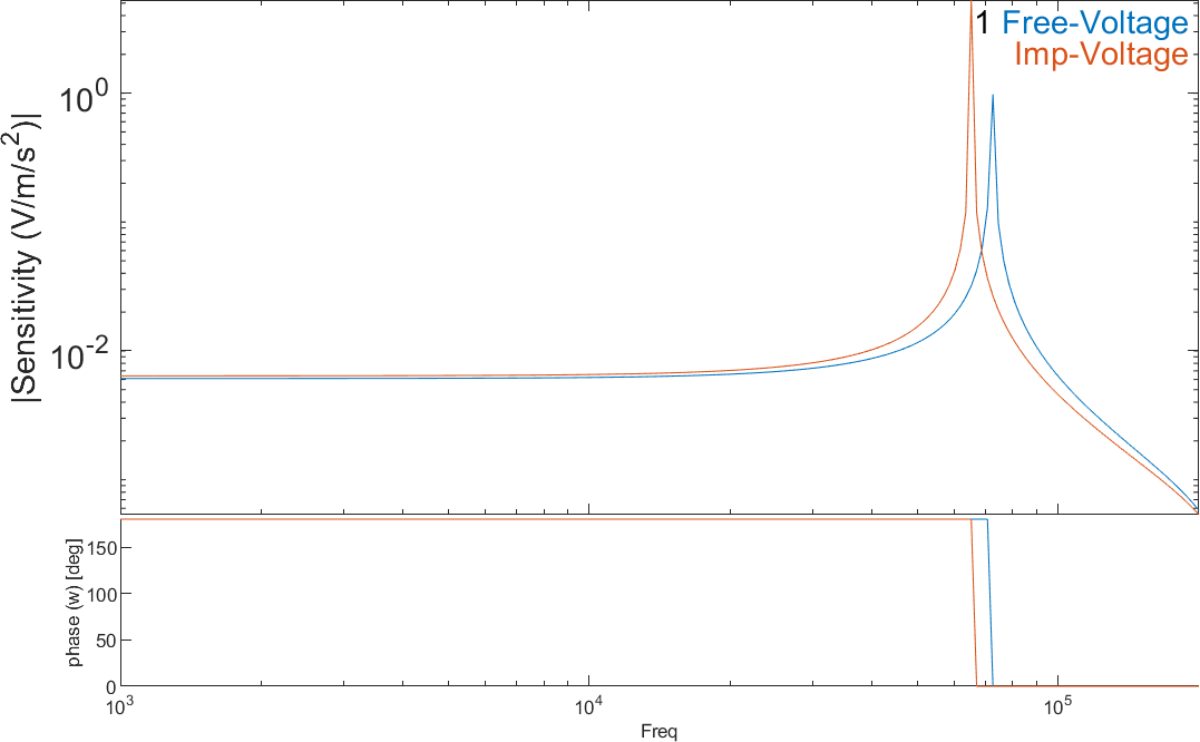
Figure 2.42: Comparison of the sensitivities computed with a uniform base acceleration, and a uniform base pressure
The sensor can also be used in the charge mode. The following scripts compares the sensitivity of the sensor used in the voltage and charge
modes. The sensitivities are normalized to the static sensitivity in order to be compared on the same graph, as the orders of magnitude are very different (Figure 2.43). The charge sensor corresponds to a short-circuit condition which results in a lower resonant frequency than the sensor used in a voltage mode where the electric field is present in the piezoelectric material which results in a stiffening due to the piezoelectric coupling, as already illustrated in Section 2.2 for a plate. Here the difference of eigenfrequency is however higher (about 10%) due to the fact that there is more strain energy in the piezoelectric element, and that it is used in the d33 mode which has a higher electromechanical coupling factor than the d31 mode.
(d_piezo('TutoAccel-s5')
)
%% Step 5 - Compare charge and voltage mode for sensing
 % Meshing script,open with sdtweb d_piezo('MeshBaseAccel')
model=d_piezo('MeshBaseAccel');
model=fe_case(model,'remove','V-Top sensor');

% Short-circuit electrodes of accelerometer
model=fe_case(model,'FixDof','V=0 on Top Sensor', ...
    p_piezo('electrodedof Top sensor',model));

% Other parameters
  model=stack_set(model,'info','Freq',logspace(3,5.3,200)');

% Link dofs of base and impose unit vertical displacement
n1=feutil('getnode z==0',model);
rb=feutilb('geomrb',n1,[0 0 0],fe_c(feutil('getdof',model),n1(:,1),'dof'));
rb=fe_def('subdef',rb,3); % Keep vertical displacement
model=fe_case(model,'DofSet','Base',rb);

 % compute
 ofact('silent'); model.DOF=[]; d1=fe_simul('dfrf',model);

 % Project on sensor and create output
 sens=fe_case(model,'sens');
 C4=fe_case('SensObserve -DimPos 2 3 1',sens,d1);
 C4.name='DFRF';C4.Ylab='Imp-displ';

 % Build a clean "curve" for iiplot display
 C4.X{2}={'Sensor output(C)';'Base Acc(m/s^2)';'Sensitivity (C/m/s^2)'};
 C4.XLab{3}='Freq [Hz]';
 C4.Y(:,2)=C4.Y(:,2).*(-(C4.X{1}*2*pi).^2); % Base acc
 C4=sdsetprop(C4,'PlotInfo','sub','magpha','show','abs','scale','xlog;ylog');
 C4.Y(:,3)=C4.Y(:,1)./C4.Y(:,2);% Sensitivity
 C4.name='Imp-Charge';

 % Normalize the sensitivities to plot on same graph
 C6=C2; % save C6 as non-normalized
 C2.Y(:,3)=C2.Y(:,3)./C2.Y(1,3);C4.Y(:,3)=C4.Y(:,3)./C4.Y(1,3);
 C2=feutil('rmfield',C2,'Ylab'); C4=feutil('rmfield',C4,'Ylab');
 iicom(ci,'curvereset');
 iicom(ci,'curveinit',{'curve',C2.name,C2;'curve',C4.name,C4});
 iicom('ch 3'); iicom('submagpha');
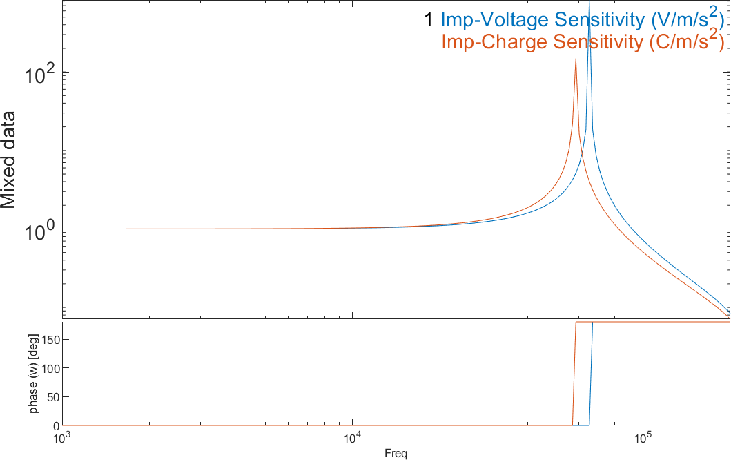
Figure 2.43: Comparison of the normalized sensitivities of the sensor used in the charge and voltage mode
Experimentally, the sensitivity curve can be measured by attaching the accelerometer to a shaker in order to excite the base. Usually, this is done with an electromagnetic shaker, but we illustrate in the following example the use of a piezoelectric shaker for sensor calibration. The piezoelectric shaker consists of two steel cylindrical parts with a piezoelectric disc inserted in between. The base of the shaker is fixed and the piezoelectric element is used as an actuator: imposing a voltage difference between the electrodes results in the motion of the top surface of the shaker to which the accelerometer is attached (Figure 2.44).
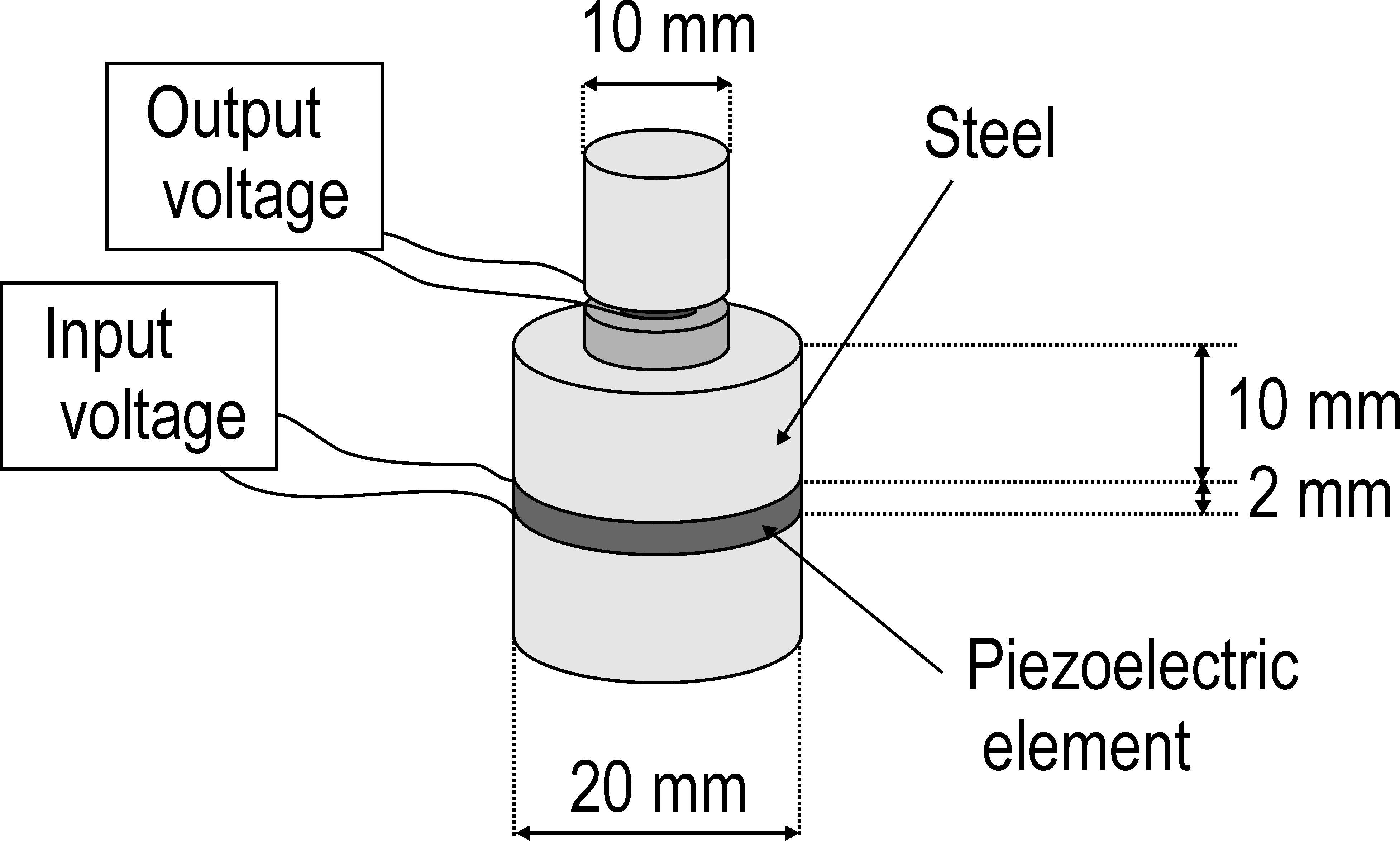
Figure 2.44: Piezoelectric accelerometer attached to a piezoelectric shaker for sensor calibration
The piezoelectric properties for the actuating element in the piezoelectric shaker are identical to the ones of the sensing element given in Table 2.6 and it is poled through the thickness. A voltage is applied to the actuator and the resulting voltage on the sensing element is computed. The sensitivity is then computed by dividing the sensor response by the acceleration at the center of the wear plate as a function of the excitation frequency. The mesh is represented in Figure 2.45 and is obtained with:
(d_piezo('TutoAcc_shaker-s1')
)
% See full example as MATLAB code in d_piezo('ScriptTutoAcc_Shaker')
%% Step 1 - Build mesh and visualize
% Meshing script,open with sdtweb d_piezo('MeshPiezoShaker')
model=d_piezo('MeshPiezoShaker');
cf=feplot(model); fecom('colordatapro');
set(gca,'cameraposition',[-0.0604   -0.0787    0.0139])
In the meshing script, a voltage actuator is defined for the piezoelectric disk in the piezo shaker by setting the bottom electrode potential to zero,
and defining the top electrode potential as an input:
(d_piezo('TutoAcc_shaker-s2')
)
%% Step 2 - Define actuators and sensors
  % -input "In" says it will be used as a voltage actuator
model=p_piezo('ElectrodeMPC Top Actuator -input "Vin-Shaker"',model,'z==-0.01');
  % -ground generates a v=0 FixDof case entry
model=p_piezo('ElectrodeMPC Bottom Actuator -ground',model,'z==-0.012');
and the shaker is mechanically attached at the bottom.
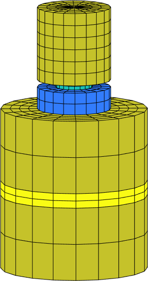
Figure 2.45: Mesh of the piezoelectric accelerometer attached to a piezoelectric shaker
After meshing, the script to obtain the sensitivity is:
% Voltage sensor will be used - remove charge sensor
model=fe_case(model,'remove','Q-Top sensor');

% Frequencies for computation
model=stack_set(model,'info','Freq',logspace(3,5.3,200)');
(d_piezo('TutoAcc_shaker-s3')
)
 %% Step 3 - Compute response, voltage input on shaker
 ofact('silent'); model.DOF=[]; d1=fe_simul('dfrf',model);

 % Project on sensor and create output
 sens=fe_case(model,'sens');
 C5=fe_case('SensObserve -DimPos 2 3 1',sens,d1);
 C5.name='DFRF';C5.Ylab='Shaker-Exc';

 % Build a clean "curve" for iiplot display
 C5.X{2}={'Sensor output(V)';'Base Acc(m/s^2)';'Sensitivity (V/m/s^2)'};
 C5.Xlab{1}='Freq [Hz]';
 C5.Y(:,2)=C5.Y(:,2).*(-(C5.X{1}*2*pi).^2); % Base acc
 C5=sdsetprop(C5,'PlotInfo','sub','magpha','show','abs','scale','xlog;ylog');
 C5.Y(:,3)=C5.Y(:,1)./C5.Y(:,2);% Sensitivity
 C5.name='Shaker-Voltage'; ci=iiplot;
 C5=feutil('rmfield',C5,'Ylab');
 ci=iiplot;
 iicom(ci,'curveinit',C5); iicom('ch 3'); iicom('submagpha');
The sensitivity curve obtained is shown in Figure 2.46. It is comparable around the natural frequency of the accelerometer, but at low frequencies, the flat part is not correctly represented and a few spurious peaks appear at high frequencies. These differences are due to the fact that the piezoelectric shaker does not impose a uniform acceleration of the base of the sensor.
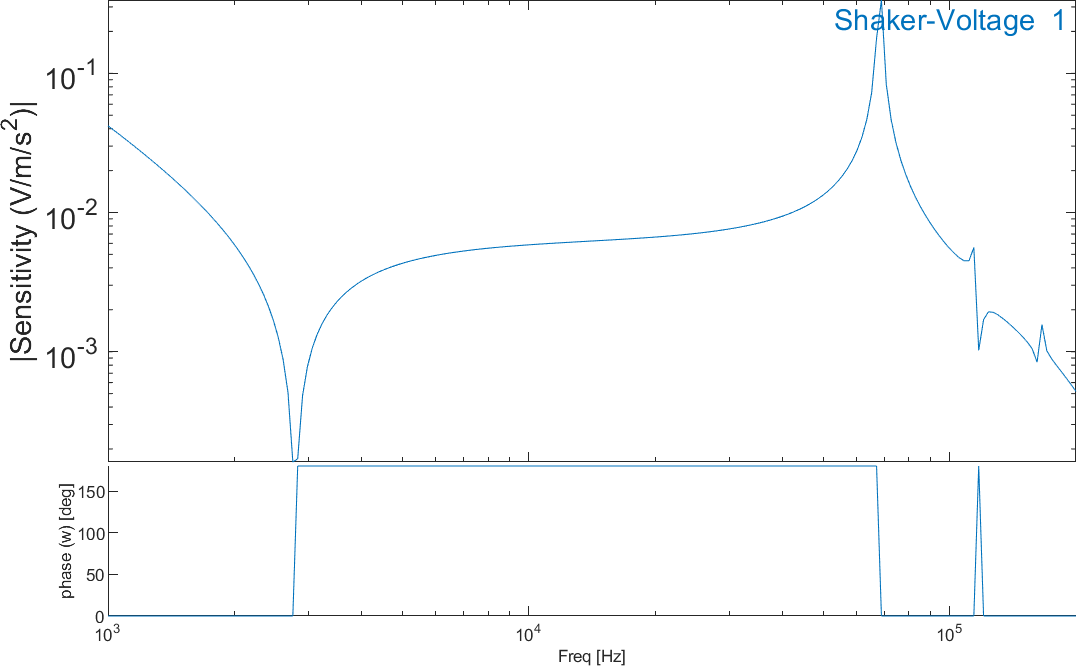
Figure 2.46: Sensitivity curve obtained with a piezoelectric shaker


