PDF Index
| SDT-piezo
Contents
Functions
PDF Index |
In this example, we will show how to compute the homogeneous equivalent mechanical, piezoelectric and dielectric properties of both P1 and P2-type MFCs. The methodology is general and can be extended to other types of piezocomposites.
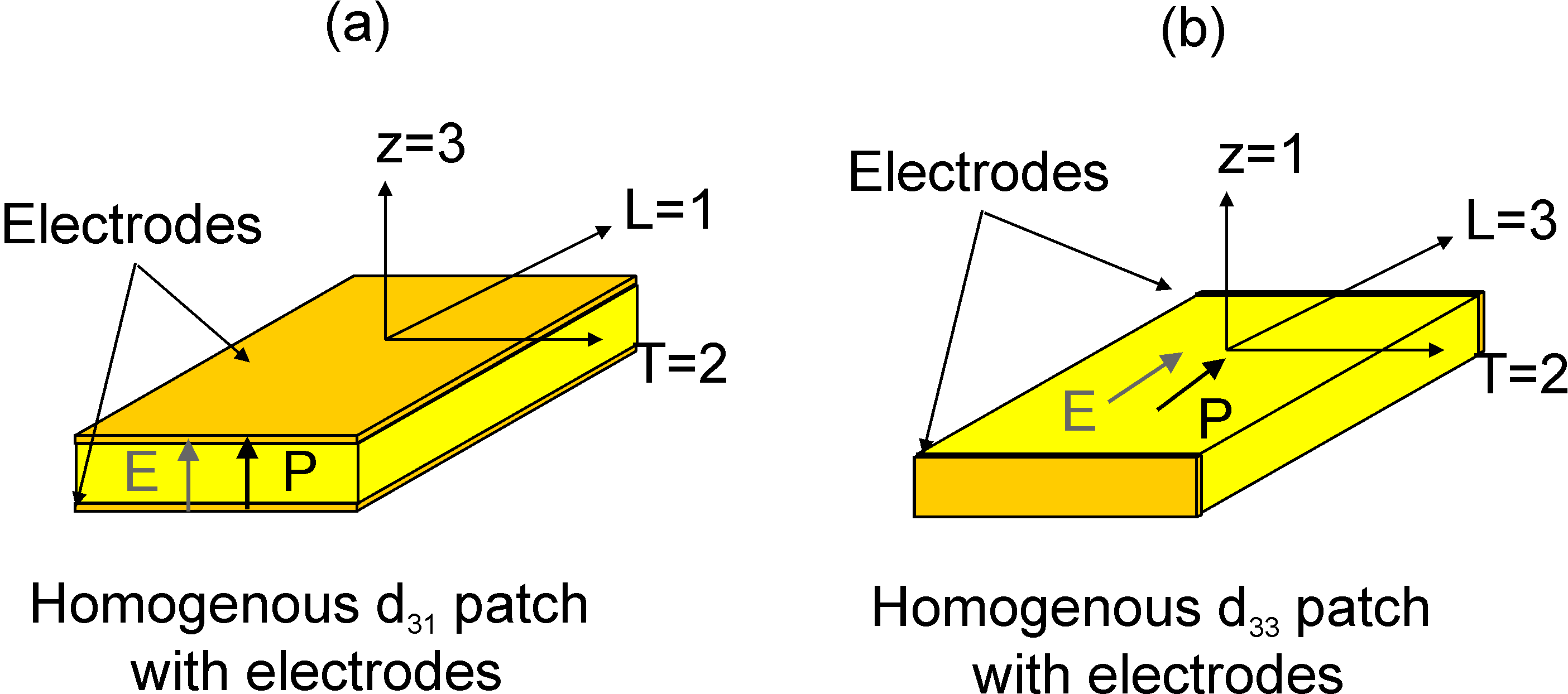
For d31 patches, the poling direction (conventionally direction 3) is normal to the plane of the patches (Figure 2.53a) and according to the plane stress assumption T3=0. The electric field is assumed to be aligned with the polarization vector (E2=E1=0). The constitutive equations reduce to:
| (19) |
where the superscript * denotes the properties under the plane stress assumption (which are not equal to the properties in 3D).
For d33 patches, although the electric field lines do not have a constant direction, when replacing the active layer by an equivalent homogeneous layer, we consider that the poling direction is that of the fibers (direction 3, Figure 2.53b), and that the electric field is in the same direction. With this reference frame, the plane stress hypothesis implies that T1=0. The constitutive equations are given by
| (20) |
Homogenization techniques are widely used in composite materials. They consist in computing the homogeneous, equivalent properties of multi-phase heterogeneous materials. The homogenization is performed on a so-called representative volume element (RVE) which is a small portion of the composite which, when repeated in 1, 2 or 3 directions forms the full composite. In the case of flat transducers considered here, the composite is periodic in 2 directions (the directions of the plane of the composite) Equivalent properties are obtained by writing the constitutive equations (Equation ((16)) or ((20)) in this case) in terms of the average values of Ti,Si,Di,Ei on the RVE:
| (21) |
where a denotes the average value.
For both types of piezocomposites, matrix [cE*] is a function of the longitudinal (in the direction of the fibers)
and transverse in-plane Young's moduli
(EL and ET), the in plane Poisson's ratio
νLT, the in-plane shear modulus GLT, and the two out-of-plane shear moduli GLz
and GTz. Matrix [e*] is given by
| (22) |
where
| (23) |
in the case of d31 piezocomposites and
| (24) |
in the case of d33 piezocomposites. Note that the coefficients dij are unchanged under the plane stress hypothesis.
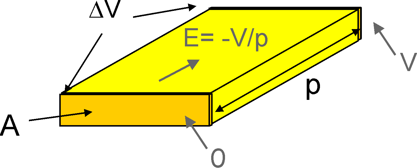
When used as sensors or actuators, piezocomposite transducers are typically equipped with two electrodes. These electrodes impose an equipotential voltage on their surfaces, and the electrical variables are the voltage difference V across the electrodes, and the electrical charge Q. These two variables are representative of the electrical macro variables which will be used in the numerical models of structures equipped with such transducers : transducers are used either in open-circuit conditions (Q=0 or imposed) or short-circuit conditions (V=0 or imposed). Instead of the average values of Di and Ei, the macro variables Q and V are therefore used in the homogenization process. For a homogeneous d33 transducer (Figure 2.54), the constitutive equations can be rewritten in terms of these macro variables:
| (25) |
where SC stands for 'short-circuit' (V=0), p is the length of the transducer, A is the surface of the electrodes of the equivalent homogeneous transducer and Q is the charge collected on the electrodes.
For d31-piezocomposites, the approach is identical.
The RVE is made of two different materials. In order to find the homogeneous constitutive equations, Equation ((25)) is written in terms of the average values of the mechanical quantities Si and Ti in the RVE and the electrical variables Q and V defined on the electrodes:
| (26) |
The different terms in Equation ((26)) can be identified by defining local problems on the RVE. The technique consists in imposing conditions on the different strain components and V and computing the average values of the stress and the charge in order to find the different coefficients. For the electric potential, two different conditions (V = 0, 1) are used. For the mechanical part, we assume that the displacement field is periodic in the plane of the transducer: on the boundary of the RVE, the displacement can be written :
| (27) |
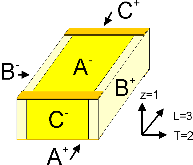
where ui is the ith component of displacement, Sij is the average strain in the RVE (tensorial notations are used), xj is the jth spatial coordinate of the point considered on the boundary, and vi is the periodic fluctuation on the RVE. The fluctuation v is periodic in the plane of the transducer so that between two opposite faces (noted A−/A+, B−/B+ and C−/C+, Figure 2.55), one can write (v(xjK+)=v(xjK−), K=A,B,C) :
| (28) |
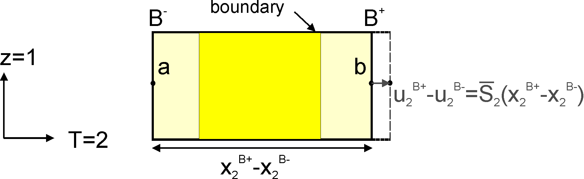
Because we consider a plate with the plane stress hypothesis T1=0, equation (28) should not be satisfied for K=A and j=1 (no constraint on the normal displacement on faces A+ and A−). For a given value of the average strain tensor (Sij), equation ((28)) defines constraints between the points on each pair of opposite faces. This is illustrated in Figure 2.56, where an average strain S2 is imposed on the RVE and the constraints are represented for u2 on faces B− and B+.
Note that these constraints do not impose that the faces of the RVE remain plane, which is important for the evaluation of the shear stiffness coefficients.
In total, six local problems are needed to identify all the coefficients in ((26)) (Figure 2.57). The first problem consists in applying a difference of potential V to the electrodes of the RVE and imposing zero displacement on all the faces (except the top and bottom). In the next five local problems, the difference of potential is set to 0 (short-circuited condition), and five deformation mechanisms are induced. Each of the deformation mechanisms consists in a unitary strain in one of the directions (with zero strain in all the other directions). For each case, the average values of Ti and Si, and the charge accumulated on the electrodes Q, are computed, and used to determine all the coefficients in ((26)), from which the engineering constants are determined.
We are going to compute the homogeneous properties of a P2-type MFC with varying volume fraction of piezoelectric fibers. We first define the range
of volume fractions to compute the homogeneous properties and the dimensions of the RVE.
( d_piezo('TutoPz_P2_homo-s1')
)
d_piezo('TutoPz_P2_homo-s1')
)
% See full example as MATLAB code in d_piezo('ScriptTutoMFC_P2_homo')
%% Step 1 - Meshing of RVE
% Meshing script can be viewed with sdtweb d_piezo('MeshHomoMFCP2')
Range=fe_range('grid',struct('rho',[0.001 linspace(0.1,0.9,9) .999], ...
  'lx',.300,'ly',.300,'lz',.180,'dd',0.04));
Then for each value of the volume fraction of piezoelectric fibers ρ, we compute the solution of the six local problems,
the average value of stress, strain and charge. From these values we extract the engineering mechanical properties, the piezoelectric
and dielectric properties.
(d_piezo('TutoPz_P2_homo-s2')
)
%% Step 2 - Loop on volume fraction and compute homogenize properties
for jPar=1:size(Range.val,1)

RO=fe_range('valCell',Range,jPar,struct('Table',2));% Current experiment

% Create mesh
model= ...
d_piezo(sprintf(['meshhomomfcp2 rho=%0.5g lx=%0.5g ly=%0.5g' ...
  'lz=%0.5g dd=%0.5g'],[RO.rho RO.lx RO.ly RO.lz RO.dd]));


% Define the six local problems
RB=struct('CellDir',[max(model.dx) max(model.dy) max(model.dz)],'Load', ...
       {{'e11','e22','e12','e23','e13','vIn'}});
 % Periodicity on u,v,w on x and y face
 % periodicity on u,v only on the z face
  RB.DirDofInd={[1:3 0],[1:3 0],[1 2 0 0]};
 % Voltage DOFs are always eliminated from periodic conditions

 % Compute the deformation for the six local problems
 def=fe_homo('RveSimpleLoad',model,RB);
 % Represent the deformation of the RVE
 cf=comgui('guifeplot-reset',2);cf=feplot(model,def); fecom('colordatamat')
% Compute stresses, strains and electric field
a1=p_piezo('viewstrain -curve -mean -EltSel MatId1 reset',cf); % Strain epoxy
a2=p_piezo('viewstrain -curve -mean -EltSel MatId2 reset',cf); % Strain piezo
b1=p_piezo('viewstress -curve -mean- EltSel MatId1 reset',cf); % Stress epoxy
b2=p_piezo('viewstress -curve -mean- EltSel MatId2 reset',cf); % Stress piezo

% Compute charge on electrodes
 mo1=cf.mdl.GetData;
  i1=fe_case(mo1,'getdata','Top Actuator');i1=fix(i1.InputDOF);
  mo1=p_piezo('electrodesensq TopQ2',mo1,struct('MatId',2,'InNode',i1));
  mo1=p_piezo('electrodesensq TopQ1',mo1,struct('MatId',1,'InNode',i1));
  c1=fe_case('sensobserve',mo1,'TopQ1',cf.def); q1=c1.Y;
  c2=fe_case('sensobserve',mo1,'TopQ2',cf.def); q2=c2.Y;


% Compute average values:
a0=a1.Y(1:6,:)*(1-RO.rho)+a2.Y(1:6,:)*RO.rho;
b0=b1.Y(1:6,:)*(1-RO.rho)+b2.Y(1:6,:)*RO.rho;
q0=q1+q2; % Total charge is the sum of charges on both parts of electrode


% Compute C matrix
C11=b0(1,1)/a0(1,1); C12=b0(1,2)/a0(2,2); C22=b0(2,2)/a0(2,2);
C44=b0(4,4)/a0(4,4); C55=b0(5,5)/a0(5,5); C66=b0(6,3)/a0(6,3);
sE=inv([C11 C12; C12 C22]);

% Extract mechanical engineering constants
E1(jPar)=1/sE(1,1); E2(jPar)=1/sE(2,2); nu12(jPar)=-sE(1,2)*E1(jPar);
nu21(jPar)=-sE(1,2)*E2(jPar);G12(jPar)=C66; G23(jPar)=C44; G13(jPar)=C55;

% Extract piezoelectric properties
e31(jPar)=b0(1,6)*RO.lz; e32(jPar)=b0(2,6)*RO.lz;
d=[e31(jPar) e32(jPar)]*sE; d31(jPar)=d(1); d32(jPar)=d(2);

% Extract dielectric properties
eps33(jPar)=-q0(6)*RO.lz/(RO.lx*RO.ly);
eps33t(jPar)=eps33(jPar)+ [d31(jPar) d32(jPar)]*[e31(jPar); e32(jPar)];

end % Loop on rho0 values
Figure 2.58 represents the solution of the six local problems for ρ=0.6.
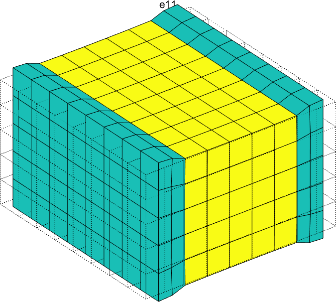
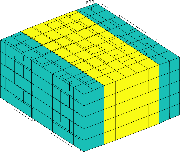
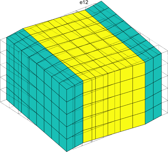
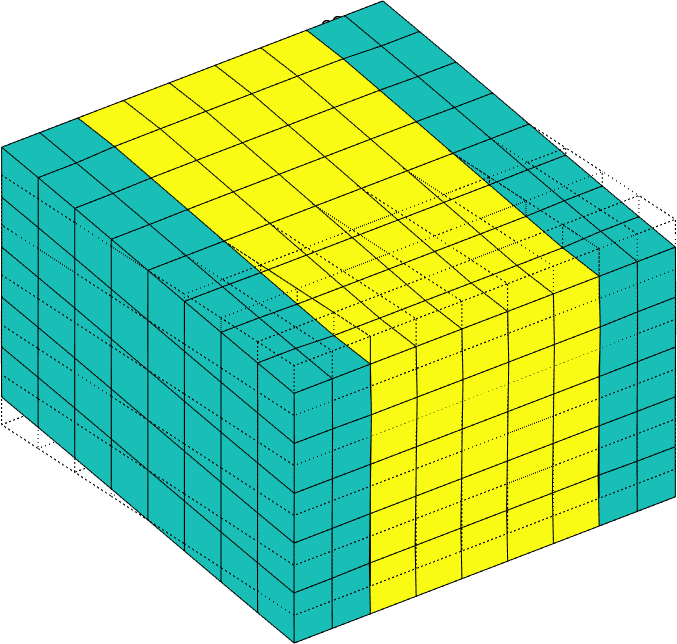
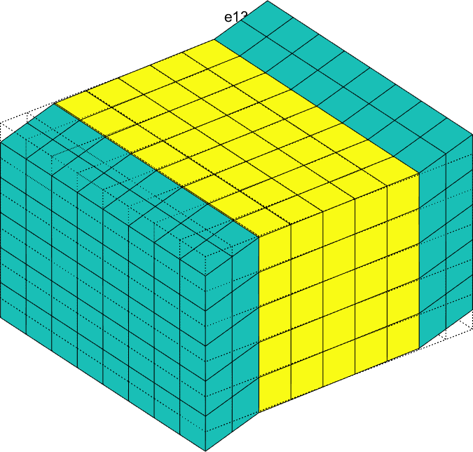
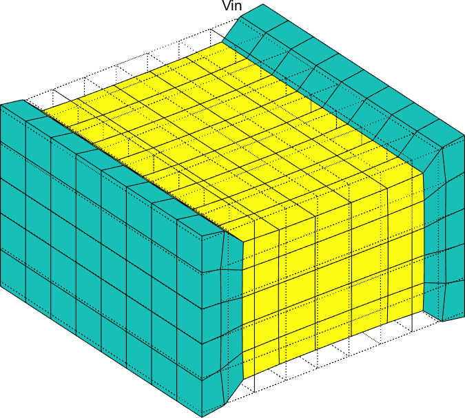
Figure 2.58: Solutions of the six local problems on the RVE for ρ=0.6 for a P2-type MFC
We can now plot the evolution of the homogeneous properties of the P2-type MFC as a function of the volume fraction ρ:
(d_piezo('TutoPz_P2_homo-s3')
)
%% Step 3 - Homogeneous properties as a function of volume fraction
rho0=Range.val(:,strcmpi(Range.lab,'rho'));

out=struct('X',{{rho0,{'E_T','E_L','nu_{LT}','G_{LT}','G_{Tz}','G_{Lz}', ...
    'e_{31}','e_{32}','d_{31}','d_{32}','epsilon_{33}^T'}'}},'Xlab',...
    {{'\rho','Component'}},'Y',[E1' E2' nu21' G12' G13' G23' e32' e31' ...
    d32' d31' eps33t'/8.854e-12]);
ci=iiplot; iicom('CurveReset');
iicom(ci,'CurveInit','P2-MFC homogenization',out);
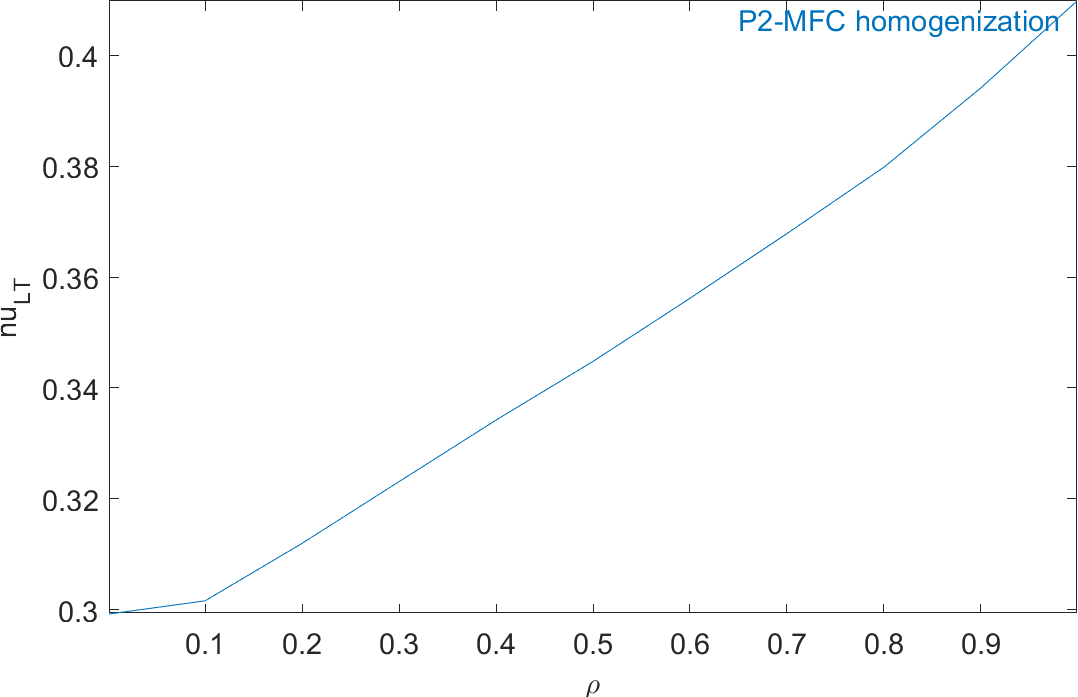
Figure 2.59 represents the evolution of the mechanical properties and Figure 2.60 represents the evolution of the piezoelectric and dielectric properties as a function of ρ. The properties of MFC transducers correspond to the value of ρ=0.86.
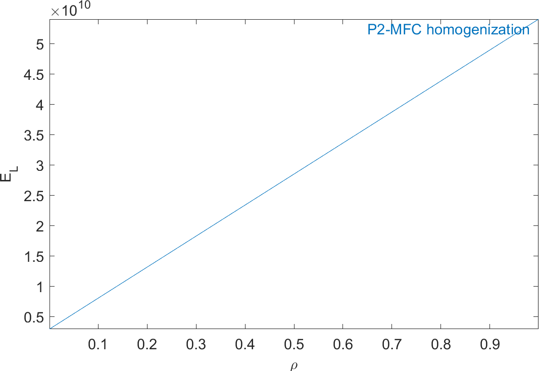
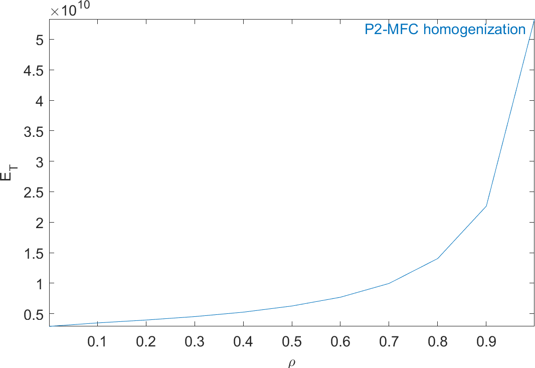

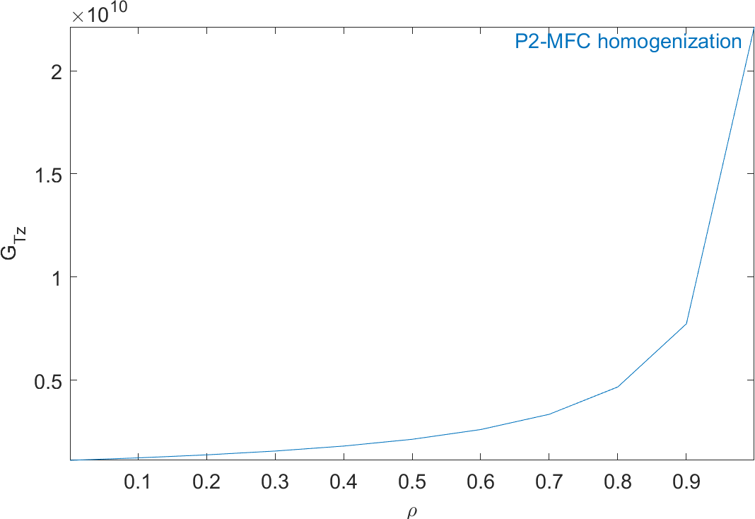
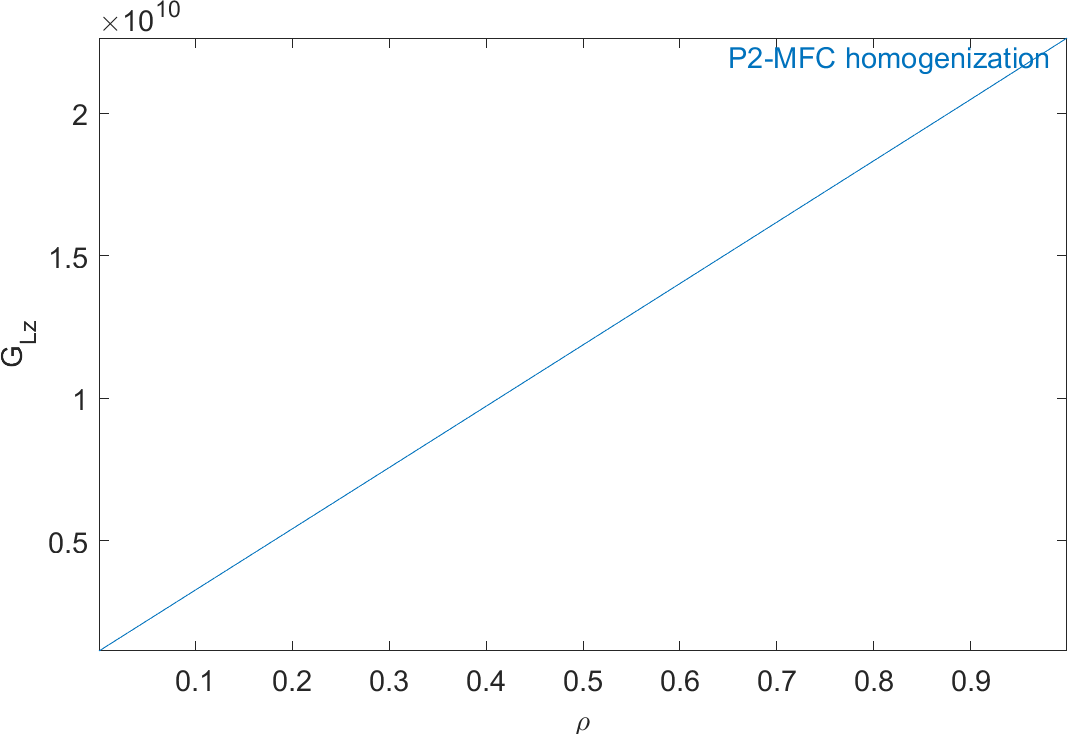
Figure 2.59: Evolution of the homogeneous mechanical properties of a P2-type piezocomposite as a function of ρ
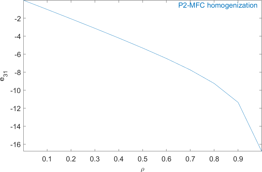
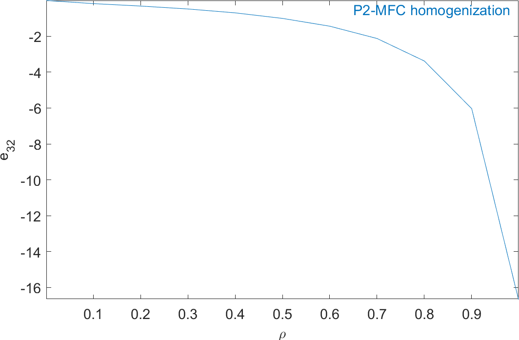
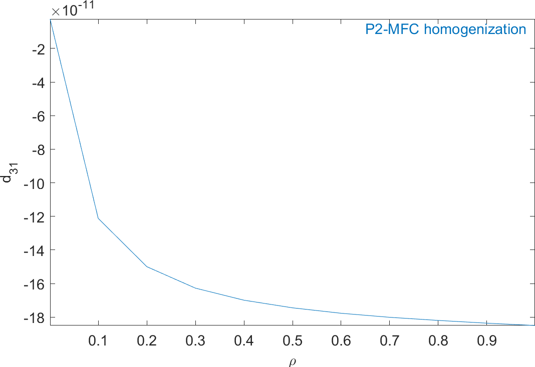
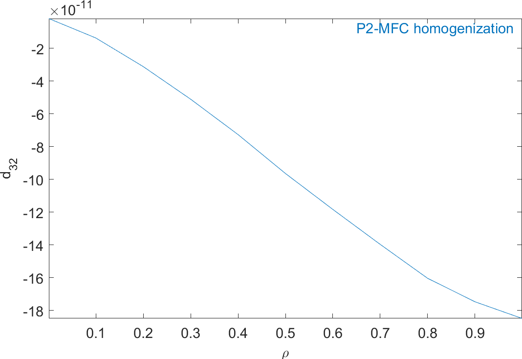
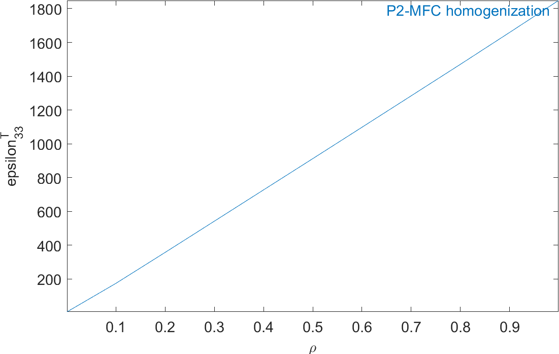
Figure 2.60: Evolution of the homogeneous piezoelectric and dielectric properties of a P2-type piezocomposite as a function of ρ
We are now going to compute the homogeneous properties of a P1-type MFC with varying volume fraction of piezoelectric fibers. We first define the range
of volume fractions to compute the homogeneous properties and the dimensions of the RVE.
(d_piezo('TutoPz_P1_homo-s1')
)
% See full example as MATLAB code in d_piezo('ScriptTutoMFC_P1_homo')
%% Step 1 - Meshing or RVE and definition of volume fractions
% Meshing script can be viewed with sdtweb d_piezo('MeshHomoMFCP1')
Range=fe_range('grid',struct('rho',[0.001 linspace(0.1,0.9,9) .999], ...
  'lx',.18,'ly',.18,'lz',1.080,'e',0.09,'dd',0.04));
Then for each value of the volume fraction of piezoelectric fibers ρ, we compute the solution of the six local problems,
the average value of stress, strain and charge. From these values we extract the engineering mechanical properties, the piezoelectric
and dielectric properties.
(d_piezo('TutoPz_P1_homo-s2')
)
%% Step 2 - Loop on volume fractions and computation of homogenized properties
for jPar=1:size(Range.val,1)

RO=fe_range('valCell',Range,jPar,struct('Table',2));% Current experiment

% Create mesh
model=...
d_piezo(sprintf(['meshhomomfcp1 rho=%0.5g lx=%0.5g ly=%0.5g lz=%0.5g' ...
   ' e=%0.5g dd=%0.5g'],[RO.rho RO.lx RO.ly RO.lz RO.e RO.dd]));

%%
RB=struct('CellDir',[max(model.dx) max(model.dy) max(model.dz)],'Load', ...
           {{'e33','e11','e23','e12','e13','vIn'}});
 % It seems fe_homo reorders the strains
 % Periodicity on u,v,w on x and z face
 % periodicity on u,w only on the y face
 % Voltage DOFs are always eliminated from periodic conditions
 RB.DirDofInd={[1:3 0],[1 0 3 0],[1:3 0]};
 def=fe_homo('RveSimpleLoad',model,RB);

cf=comgui('guifeplot-reset',2);
cf=feplot(model,def); fecom('colordatamat'); fecom('triax')
% Electric field for Vin
p_piezo('electrodeview -fw',cf); % to see the electrodes on the mesh
cf.sel(1)={'groupall','colorface none -facealpha0 -edgealpha.1'};
p_piezo('viewElec EltSel "matid1:2" DefLen 0.07 reset',cf);
fecom('scd 1e-10')
% Compute stresses, strains and electric field
a1=p_piezo('viewstrain -curve -mean -EltSel MatId1 reset',cf); % Strain S epoxy
a2=p_piezo('viewstrain -curve -mean -EltSel MatId2 reset',cf); % Strain S piezo
b1=p_piezo('viewstress -curve -mean- EltSel MatId1 reset',cf); % Stress T
b2=p_piezo('viewstress -curve -mean- EltSel MatId2 reset',cf); % Stress T

% Compute charge
 mo1=cf.mdl.GetData;
  i1=fe_case(mo1,'getdata','Top Actuator');i1=fix(i1.InputDOF);
  mo1=p_piezo('electrodesensq TopQ2',mo1,struct('MatId',2,'InNode',i1));
  mo1=p_piezo('electrodesensq TopQ1',mo1,struct('MatId',1,'InNode',i1));
  c1=fe_case('sensobserve',mo1,'TopQ1',cf.def); q1=c1.Y;
  c2=fe_case('sensobserve',mo1,'TopQ2',cf.def); q2=c2.Y;

% Compute average values:
a0=a1.Y(1:6,:)*(1-RO.rho)+a2.Y(1:6,:)*RO.rho;
b0=b1.Y(1:6,:)*(1-RO.rho)+b2.Y(1:6,:)*RO.rho;
q0=q1+q2; %total charge is the sum of charges

% Compute C matrix
C11=b0(3,2)/a0(3,2); C12=b0(3,1)/a0(1,1); C22=b0(1,1)/a0(1,1);
C44=b0(5,5)/a0(5,5); C55=b0(4,4)/a0(4,4); C66=b0(6,3)/a0(6,3);
sE=inv([C11 C12; C12 C22]);
E1(jPar)=1/sE(1,1); E2(jPar)=1/sE(2,2); nu12(jPar)=-sE(1,2)*E1(jPar);
nu21(jPar)=-sE(1,2)*E2(jPar);
e33(jPar)=b0(3,6)*RO.lz;
e31(jPar)=b0(1,6)*RO.lz;
eps33(jPar)=-q0(6)*RO.lz/(RO.ly*RO.lx);
d=[e33(jPar) e31(jPar)]*sE; d33(jPar)=d(1); d31(jPar)=d(2);
eps33t(jPar)=eps33(jPar)+ [d33(jPar) d31(jPar)]*[e33(jPar); e31(jPar)];
G12(jPar)=C44;
G23(jPar)=C66;
G13(jPar)=C55;

end % loop on Rho values
Figure 2.61 represents the solution of the six local problems for ρ=0.6.

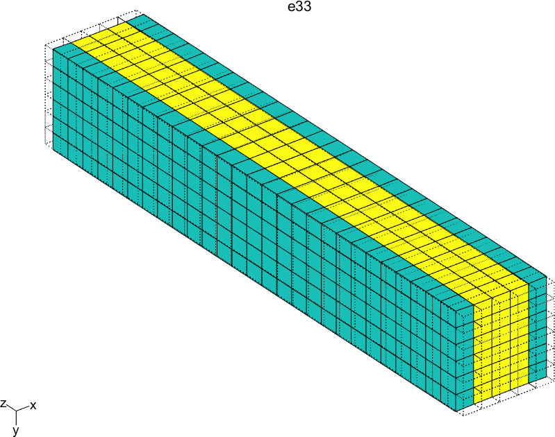
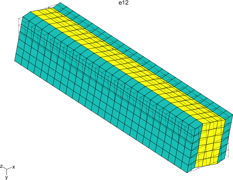

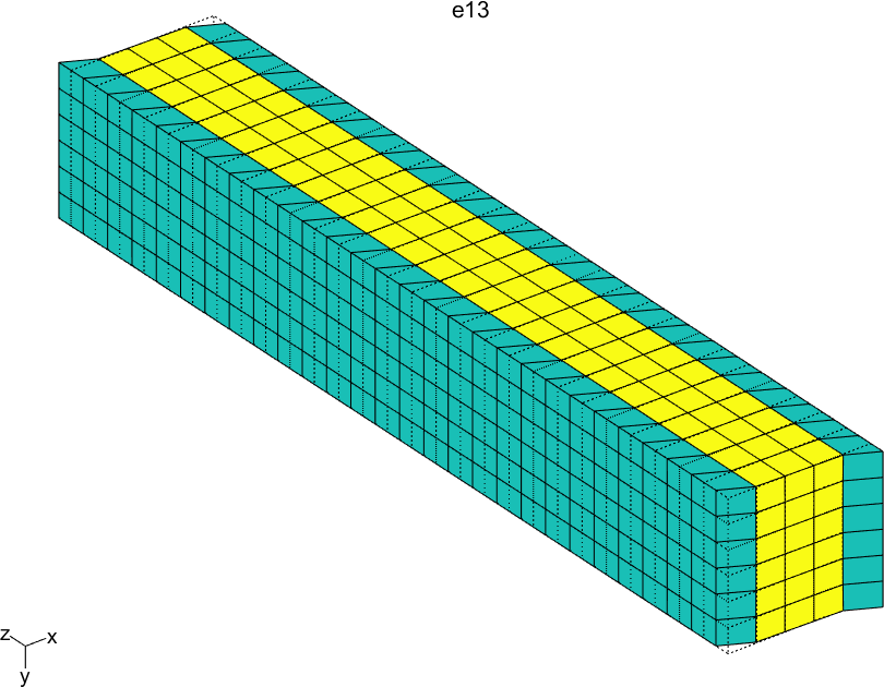

Figure 2.61: Solutions of the six local problems on the RVE for ρ=0.6
Figure 2.62 represents the inhomogeneous electric field for the sixth local problem (applied voltage) and ρ=0.6.
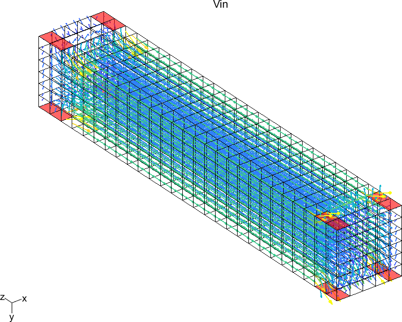
Figure 2.62: Electric field for the sixth local problem (applied voltage) on the RVE of a P1-type MFC for ρ=0.6
We can now plot the evolution of the homogeneous properties of the P1-type MFC as a function of the volume fraction ρ
(d_piezo('TutoPz_P1_homo-s3')
)
%% Step 3 - Plot homogeneous properties as a function of volume fraction
rho0=Range.val(:,strcmpi(Range.lab,'rho'));

out=struct('X',{{rho0,{'E_L','E_T','nu_{LT}','G_{LT}','G_{Lz}','G_{Tz}', ...
    'e_{31}','e_{33}','d_{31}','d_{33}','epsilon_{33}^T'}'}},'Xlab',...
    {{'\rho','Component'}},'Y',[E1' E2' nu12' G12' G13' G23' e31' e33' ...
    d31' d33' eps33t'/8.854e-12]);
ci=iiplot;
iicom('CurveReset');
iicom(ci,'CurveInit','P1-MFC homogenization',out);
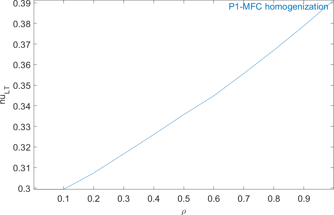
Figure 2.63 represents the evolution of the mechanical properties and Figure 2.64 represents the evolution of the piezoelectric and dielectric properties as a function of ρ. The properties of MFC transducers correspond to the value of ρ=0.86.
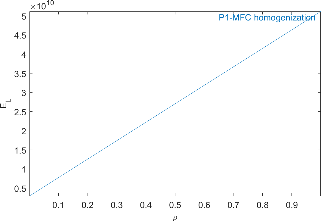
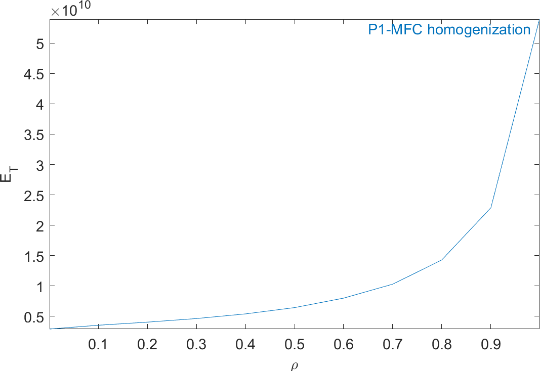
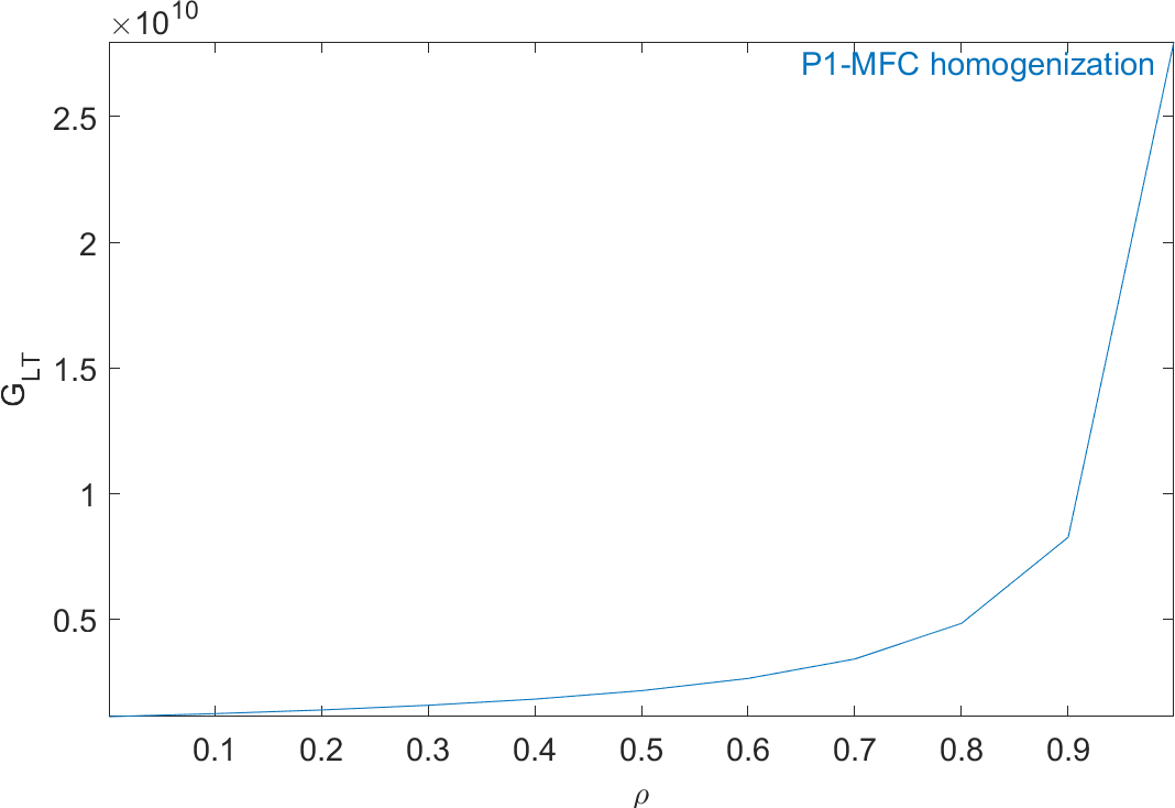
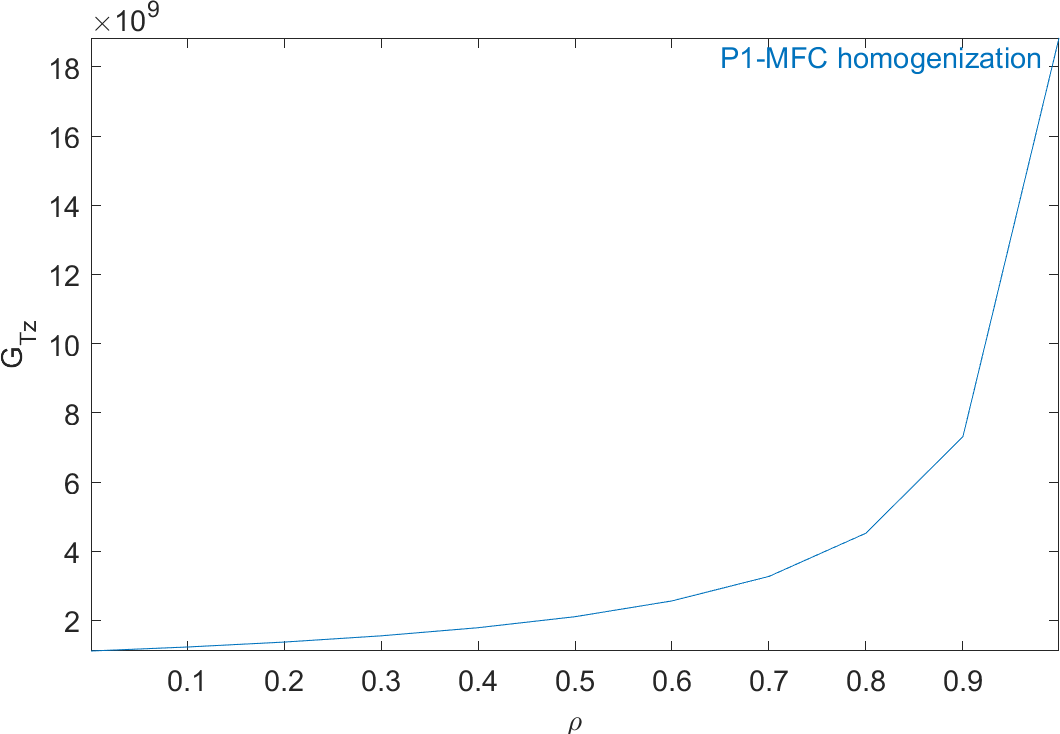
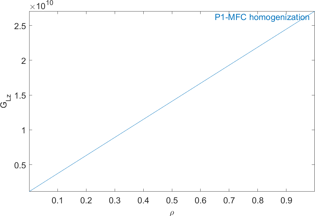
Figure 2.63: Evolution of the homogeneous mechanical properties of a P1-type piezocomposite as a function of ρ
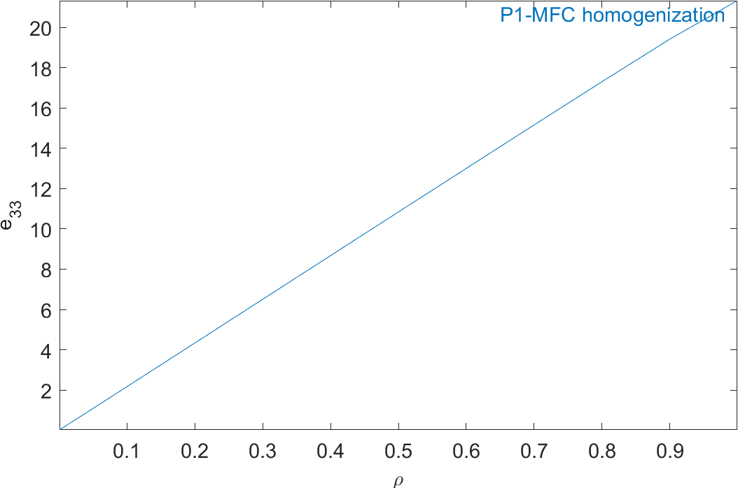
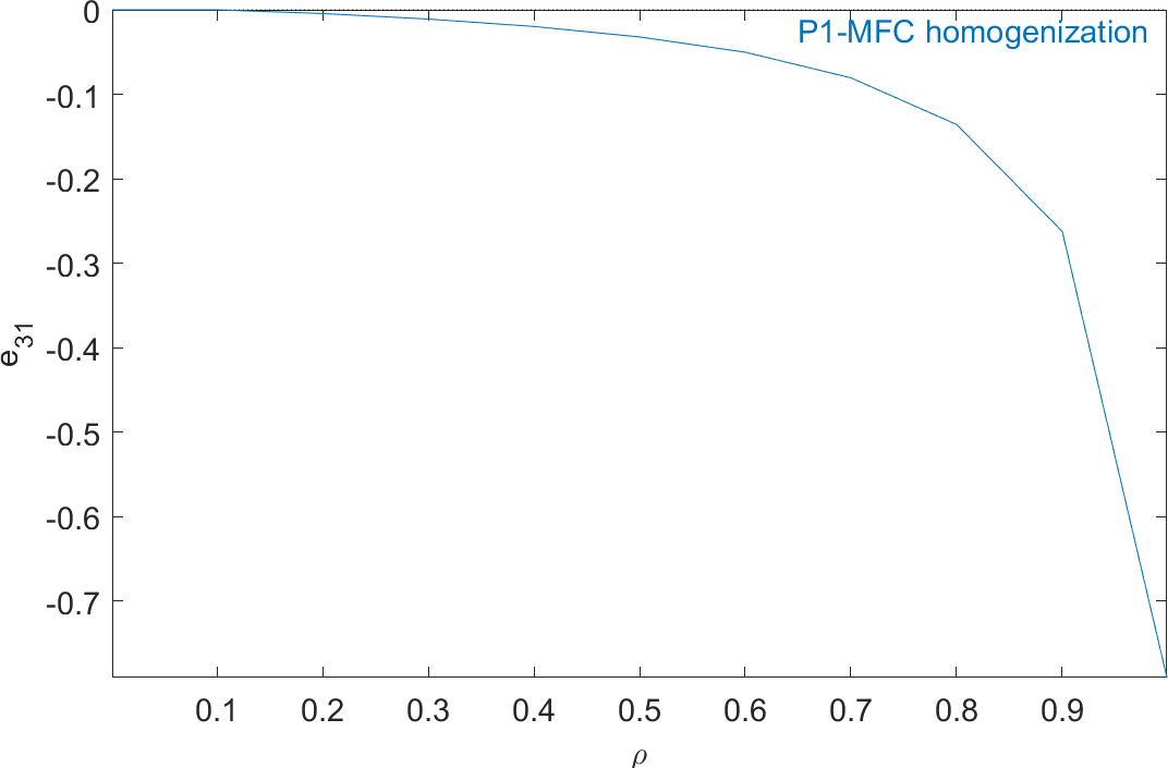
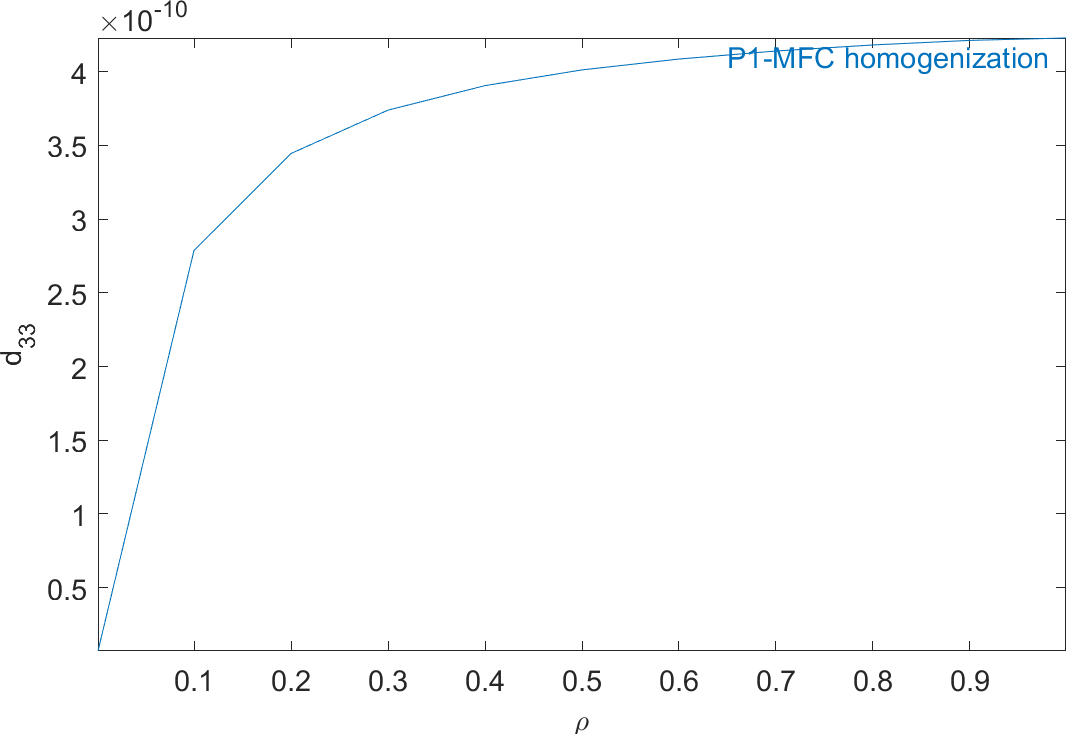
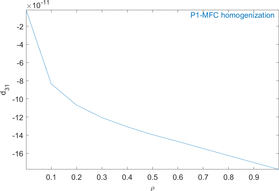
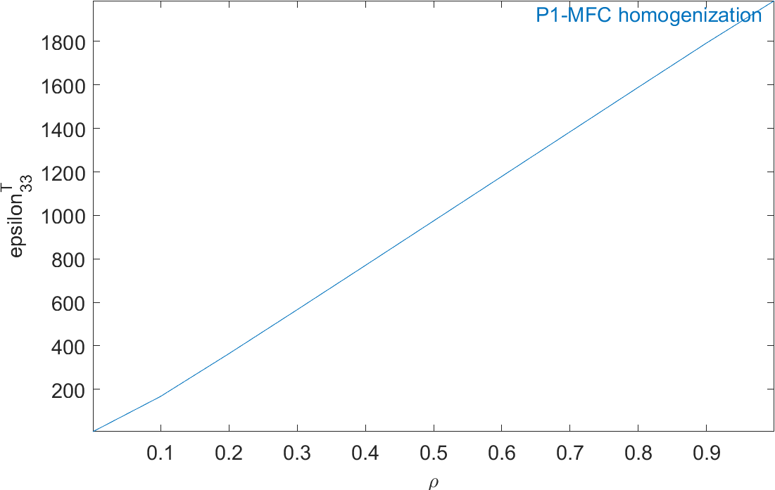
Figure 2.64: Evolution of the homogeneous piezoelectric and dielectric properties of a P1-type piezocomposite as a function of ρ
All the properties match well the results presented in []