I/O shape matrices

Contents Functions

5.1 I/O shape matrices

Dynamic loads applied to a discretized mechanical model can be decomposed into a product {F}_q= [b] {u(t)} where

the input shape matrix [b] is time invariant and characterizes spatial properties of the applied forces
the vector of inputs {u} allows the description of the time/frequency properties.

Similarly it is assumed that the outputs {y} (displacements but also strains, stresses, etc.) are linearly related to the model coordinates {q} through the sensor output shape matrix ({y} = [c] {q}).

Input and output shape matrices are typically generated with fe_c or fe_load. Understanding what they represent and how they are transformed when model DOFs/states are changed is essential.

Linear mechanical models take the general forms

[Ms²+Cs+K]_N × N {q(s)} = [b]_N × NA {u(s)}_NA × 1

{y(s)}_NS × 1 = [c]_NS × N {q(s)}_N × 1

(5.1)

in the frequency domain (with Z(s)=Ms²+Cs+K), and

[M] {q} + [C] {q} + [K] {q} = [b]{u(t)}

{y(t)}= [c] {q(t)}

(5.2)

in the time domain.

In the model form (5.1), the first set of equations describes the evolution of {q}. The components of q are called Degrees Of Freedom (DOFs) by mechanical engineers and states in control theory. The second observation equation is rarely considered by mechanical engineers (hopefully the SDT may change this). The purpose of this distinction is to lead to the block diagram representation of the structural dynamics

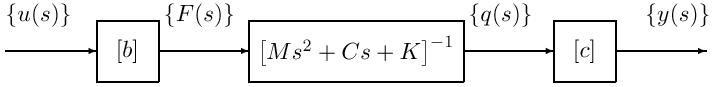
which is very useful for applications in both control and mechanics.

In the simplest case of a point force input at a DOF q_l, the input shape matrix is equal to zero except for DOF l where it takes the value 1

[b_l] = [

⋮

]

← l

(5.3)

Since {q_l} = [b_l]^T {q}, the transpose this Boolean input shape matrix is often called a localization matrix. Boolean input/output shape matrices are easily generated by fe_c (see the section on DOF selection ).

Input/output shape matrices become really useful when not Boolean. For applications considered in the SDT they are key to

distributed FEM loads, see fe_load.
test analysis correlation. Since you often have measurements that do not directly correspond to DOFs (accelerations in non global directions at positions that do not correspond to finite element nodes, see section 2.2.2).
model reduction. To allow the changes to the DOFs q while retaining the physical meaning of the I/O relation between {u} and {y} (see section 6.2).