
 PDF Index
| SDT-base
Contents
Functions
PDF Index |
Different major applications use families of structural models. Update problems, where a comparison with experimental results is used to update the mass and stiffness parameters of some elements or element groups that were not correctly modeled initially. Structural design problems, where component properties or shapes are optimized to achieve better performance. Non-linear problems where the properties of elements change as a function of operating conditions and/or frequency (viscoelastic behavior, geometrical non-linearity, etc.).
A family of models is defined (see [9] for more details) as a group of models of the general second order form (5.1) where the matrices composing the dynamic stiffness depend on a number of design parameters p
| (6.122) |
Moduli, beam section properties, plate thickness, frequency dependent damping, node locations, or component orientation for articulated systems are typical p parameters. The dependence on p parameters is often very non-linear. It is thus often desirable to use a model description in terms of other parameters α (which depend non-linearly on the p) to describe the evolution from the initial model as a linear combination (called zCoef in SDT)
| (6.123) |
with each [Zjα(s)] having constant mass, damping and stiffness properties.
Plates give a good example of p and α parameters. If p represents the plate thickness, one defines three α parameters: t for the membrane properties, t3 for the bending properties, and t2 for coupling effects.
p parameters linked to elastic properties (plate thickness, beam section properties, frequency dependent damping parameters, etc.) usually lead to low numbers of α parameters so that the α should be used. In other cases (p parameters representing node positions, configuration dependent properties, etc.) the approach is impractical and p should be used directly.
SDT handles parametric models where various areas of the model are associated with a scalar coefficient weighting the model matrices (stiffness, mass, damping, ...). The first step is to define a set of parameters, which is used to decompose the full model matrix in a linear combination.
The elements are grouped in non overlapping sets, indexed m, and using the fact that element stiffness depend linearly on the considered moduli, one can represent the dynamic stiffness matrix of the parameterized structure as a linear combination of constant matrices
| (6.124) |
Parameters are case stack entries defined by using fe_case par commands (which are identical to upcom Par commands for an upcom superelement).
A parameter entry defines a element selection and a type of varying matrix. Thus
 model=demosdt('demoubeam');
 model=fe_case(model,'par k 1 .1 10','Top','withnode {z>1}');
 fecom('proviewon');fecom('curtabCase','Top') % highlight the area
The weighting coefficients in (6.124) are defined formally using the
cf.Stack{'info','zCoef'} cell array viewed in the figure and detailed below.
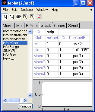
The columns of the cell array, which can be modified with the feplot interface, give
Given a model with defined parameters/matrices, model=fe_def('zcoef-default',model) defines default parameters.
zcoef=fe_def('zcoef',model) returns weighting coefficients for a range of values using the frequencies (see Freq) and design point stack entries
Frequencies are stored in the model using a call of the form model=stack_set(model,'info','Freq',w_hertz_colum). Design points (temperatures, optimization points, ...) are stored as rows of the 'info','Range' entry, see fevisco Range for generation.
When computing a response, fe_def zCoef starts by putting frequencies in a local variable w (which by convention is always in rd/s), and the current design point (row of 'info','Range' entry or row of its .val field if it exists) in a local variable par. zCoef2:end,4 is then evaluated to generate weighting coefficients zCoef giving the weighting needed to assemble the dynamic stiffness matrix (6.124). For example in a parametric analysis, where the coefficient par(1) stored in the first column of Range. One defines the ratio of current stiffness to nominal Kvcurrent=par(1)*Kv(nominal) as follows
% external to fexf
 zCoef={'Klab','mCoef','zCoef0','zCoefFcn';
        'M'    1       0        '-w.^2';
        'Ke'   0       1        1+i*fe_def('DefEta',[]);
        'Kv'   0       1        'par(1)'};
model=struct('K',{cell(1,3)});
model=stack_set(model,'info','zCoef',zCoef);
model=stack_set(model,'info','Range', ...
   struct('val',[1;2;3],'lab',{{'par'}}));

%Within fe2xf
w=[1:10]'*2*pi;  % frequencies in rad/s
Range=stack_get(model,'info','Range','getdata');
for jPar=1:size(Range.val,1)
 Range.jPar=jPar;zCoef=fe2xf('zcoef',model,w,Range);
 disp(zCoef)
  % some work gets done here ...
end
As for nominal models, parameterized models can be reduced by projection on a constant reduction basis T leading to input/output models of the form
| (6.125) |
or, using the α parameters,
| (6.126) |
Although superelements can deal with arbitrary models of the form
(6.123), the upcom interface is designed to allow easier parameterization of models. This interface stores a long list of mass Me and stiffness Ke matrices associated to each element and provides, through the assemble command, a fast algorithm to assemble the full order matrices as weighted sums of the form
| (6.127) |
where the nominal model corresponds to αk(p)=βk(p)=1.
The basic parameterizations are mass pi and stiffness pj coefficients associated to element selections ei,ej leading to coefficients
| (6.128) |
Only one stiffness and one mass parameter can be associated with each element. The element selections ei and ej are defined using upcom Par commands. In some upcom commands, one can combine changes in multiple parameters by defining a matrix dirp giving the pi,pj coefficients in the currently declared list of parameters.
Typically each element is only associated to a single mass and stiffness matrix. In particular problems, where the dependence of the element matrices on the design parameter of interest is non-linear and yet not too complicated more than one submatrix can be used for each element.
In practice, the only supported application is related to plate/shell thickness. If p represents the plate thickness, one defines three α,β parameters: t for the membrane properties, t3 for the bending properties, and t2 for coupling effects. This decomposition into element submatrices is implemented by specific element functions, q4up and q8up, which build element submatrices by calling quad4 and quadb. Triangles are supported through the use of degenerate quad4 elements.
Element matrix computations are performed before variable parameters are declared. In cases where thickness variations are desired, it is thus important to declare which group of plate/shell elements may have a variable thickness so that submatrices will be separated during the call to fe_mk. This is done using a call of the form upcom('set nominal t GroupID',FEnode,FEel0,pl,il).
Basic operation of the upcom interface is demonstrated in gartup.
The first step is the selection of a file for the superelement storage using upcom('load FileName'). If the file already exists, existing fields of Up are loaded. Otherwise, the file is created.
If the results are not already saved in the file, one then computes mass and stiffness element matrices (and store them in the file) using
upcom('setnominal',FEnode,FEelt,pl,il)
which calls fe_mk. You can of course eliminate some DOFs (for fixed boundary conditions) using a call of the form
upcom('setnominal',FEnode,FEelt,pl,il,[],adof)
At any time, upcom info will printout the current state of the model: dimensions of full/reduced model (or a message if one or the other is not defined)
 'Up' superelement (stored in '/tmp/tp425896.mat')

 Model Up.Elt with 90 element(s) in 2 group(s)
 Group 1 :    73 quad4  MatId 1 ProId 3
 Group 6 :    17 q4up  MatId 1 ProId 4

 Full order (816 DOFs, 90 elts, 124 (sub)-matrices, 144 nodes)
 Reduced model undefined
 No declared parameters
In most practical applications, the coefficients of various elements are not independent. The upcom par commands provide ways to relate element coefficients to a small set of design variables. Once parameters defined, you can easily set parameters with the parcoef command (which computes the coefficient associated to each element (sub-)matrix) and compute the response using the upcom compute commands. For example
Up=upcom('load GartUp');
Up=upcom(Up,'ParReset')
Up=upcom(Up,'ParAdd k','Tail','group3');
Up=upcom(Up,'ParAdd t','Constrained Layer','group6');
Up=upcom(Up,'ParCoef',[1.2 1.1]);
upcom(Up,'info')
cf=feplot(Up);
cf.def(1)=fe_eig(Up,[6 20 1e3]);fecom('scd.3');
The upcom interface allows the simultaneous use of a full and a reduced order model. For any model in a considered family, the full and reduced models can give estimates of all the qualities (static responses, modal frequencies, modeshapes, or damped system responses). The reduced model estimate is however much less numerically expensive, so that it should be considered in iterative schemes.
The selection of the reduction basis T is essential to the accuracy of a reduced family of models. The simplest approach, where low frequency normal modes of the nominal model are retained, very often gives poor predictions. For other bases see the discussion in section 6.2.7.
A typical application (see the gartup demo), would take a basis combining modes and modeshape sensitivities, orthogonalize it with respect to the nominal mass and stiffness (doing it with fe_norm ensures that all retained vectors are independent), and project the model
 upcom('parcoef',[1 1]);
 [fsen,mdsen,mode,freq] = upcom('sens mode full',eye(2),7:20);
 [m,k]=upcom('assemble');T = fe_norm([mdsen mode],m,k);
 upcom('par red',[T])
In the gartup demo, the time needed to predict the first 20 modes is divided by 10 for the reduced model. For larger models, the ratio is even greater which really shows how much model reduction can help in reducing computational times.
Note that the projected model corresponds to the currently declared variable parameters (and in general the projection basis is computed based on knowledge of those parameters). If parameters are redefined using Par commands, you must thus project the model again.
The upcom interface provides optimized code for the computation, at any design point, of modes (ComputeMode command), modeshape sensitivities (SensMode), frequency response functions using a modal model (ComputeModal) or by directly inverting the dynamic stiffness (ComputeFRF). All predictions can be made based on either the full or reduced order model. The default model can be changed using upcom('OptModel[0,1]') or by appending full or reduced to the main command. Thus
 upcom('ParCoef',[1 1]);
 [md1,f1] = upcom('compute mode full 105 20 1e3');
 [md2,f2] = upcom('compute mode reduced');
would be typical calls for a full (with a specification of the fe_eig options in the command rather than using the Opt command) and reduced model.
Warning: unlike fe_eig, upcom typically returns frequencies in Hz (rather than rd/s) as the default unit option is 11 (for rd/s use upcom('optunit22'))
Given modes you could compute FRFs using
IIxh = nor2xf(freq,0.01,mode'*b,c*mode,IIw*2*pi);
but this does not include a static correction for the inputs described by b. You should thus compute the FRF using (which returns modes as optional output arguments)
[IIxh,mode,freq] = upcom('compute modal full 105 20',b,c,IIw);
This approach to compute the FRF is based on modal truncation with static correction (see section 6.2.3). For a few frequency points or for exact full order results, you can also compute the response of the full order model using
IIxh = upcom('compute FRF',b,c,IIw);
In FE model update applications, you may often want to compute modal frequencies and shape sensitivities to variations of the parameters. Standard sensitivities are returned by the upcom sens command (see the Reference section for more details).


