
 PDF Index
| SDT-base
Contents
Functions
PDF Index |
The various procedures used to build the initial pole set (see step 1 above) tend to give good but not perfect approximations of the pole sets. In particular, they tend to optimize the model for a cost that differs from the broadband quadratic cost that is really of interest here and thus result in biased pole estimates.
It is therefore highly desirable to perform non-linear update of the poles in ci.Stack{'IdMain'}. This update, which corresponds to a Non-Linear Least-Squares minimization[19][18] which can be performed using different algorithms below.
The optimization problem is very non linear and non convex, good results are thus only found when improving results that are already acceptable (the result of phase 2 looks similar to the measured transfer function).
idcom eup (id_rc function) starts by reminding you of the currently selected options (accessible from the figure pointer ci.IDopt) for the type of residual corrections, model selected and, when needed, partial frequency range selected
 Low and high frequency mode correction
 Complex residue symmetric pole pattern
the algorithm then does a first estimation of residues and step directions and outputs
  %  mode#   dstep (%)     zeta      fstep (%)     freq
       1      10.000    1.0001e-02    -0.200    7.1043e+02
       2     -10.000    1.0001e-02     0.200    1.0569e+03
       3      10.000    1.0001e-02    -0.200    1.2176e+03
       4      10.000    1.0001e-02    -0.200    1.4587e+03
 Quadratic cost
    4.6869e-09
 Log-mag least-squares cost
    6.5772e+01
 how many more iterations? ([cr] for 1, 0 to exit) 30
which indicates the current pole positions, frequency and damping steps, as well as quadratic and logLS costs for the complete set of FRFs. These indications and particularly the way they improve after a few iterations should be used to determine when to stop iterating.
Here is a typical result after about 20 iterations
  %  mode#   dstep (%)     zeta      fstep (%)    freq
       1      -0.001    1.0005e-02     0.000    7.0993e+02
       2      -0.156    1.0481e-02    -0.001    1.0624e+03
       3      -0.020    9.9943e-03     0.000    1.2140e+03
       4      -0.039    1.0058e-02    -0.001    1.4560e+03
 Quadratic cost
  4.6869e-09 7.2729e-10 7.2741e-10 7.2686e-10 7.2697e-10
 Log-mag least-squares cost
  6.5772e+01 3.8229e+01 3.8270e+01 3.8232e+01 3.8196e+01
how many more iterations? ([cr] for 1, 0 to exit) 0
Satisfactory convergence can be judged by the convergence of the quadratic and logLS cost function values and the diminution of step sizes on the frequencies and damping ratios. In the example, the damping and frequency step-sizes of all the poles have been reduced by a factor higher than 50 to levels that are extremely low. Furthermore, both the quadratic and logLS costs have been significantly reduced (the leftmost value is the initial cost, the right most the current) and are now decreasing very slowly. These different factors indicate a good convergence and the model can be accepted (even though it is not exactly optimal).
The step size is divided by 2 every time the sign of the cost gradient changes (which generally corresponds passing over the optimal value). Thus, you need to have all (or at least most) steps divided by 8 for an acceptable convergence. Upon exit from id_rc, the idcom eup command displays an overlay of the measured data ci.Stack{'Test'} and the model with updated poles ci.Stack{'IdFrf'}. As indicated before, you should use the error and quality plots to see if mode tuning is needed.
The optimization is performed in the selected frequency range (idopt wmin and wmax indices). It is often useful to select a narrow frequency band that contains a few poles and update these poles. When doing so, model poles whose frequency are not within the selected band should be kept but not updated (use the euplocal and eoptlocal commands). You can also update selected poles using the 'eup num i' command (for example if you just added a pole that was previously missing).
eopt (id_rcopt function) performs a conjugate gradient optimization with a small tolerance to allow faster convergence. But, as a result, it may be useful to run the algorithm more than once. The algorithm is guaranteed to improve the result but tends to get stuck at non optimal locations.
eup(id_rc function) uses an ad-hoc optimization algorithm, that is not guaranteed to improve the result but has been found to be efficient during years of practice.
You should use the eopt command when optimizing just one or two poles (for example using eoptlocal or 'eopt num i' to optimize different poles sequentially) or if the eup command does not improve the result as it could be expected.
In many practical applications the results obtained after this first set of iterations are incomplete. Quite often local poles will have been omitted and should now be appended to the current set of poles (going back to step 1). Furthermore some poles may be diverging (damping and/or frequency step not converging towards zero). This divergence will occur if you add too many poles (and these poles should be deleted) and may occur in cases with very closely spaced or local modes where the initial step or the errors linked to other poles change the local optimum for the pole significantly (in this case you should reset the pole to its initial value and restart the optimization).
A way to limit the divergence issue is to perform sequential local updating arround each pole : one pole is updated at a time so that it is more likely to converge. This sequential optimization as been packaged for both
To pratice, the GARTEUR test case already used in previous sections is loaded with an initial set of poles by clicking on  this link
.
this link
.
Many strategies can be used to perform the optimization. In the following tutorial, we only propose to guide you through the use of some optimization steps, but the reader is encouraged to test local, broadband, narrowband strategies as he whish to better understand their strengths and weaknesses.
Run
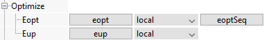
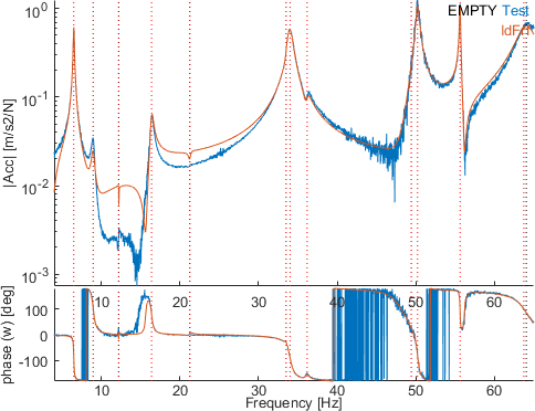
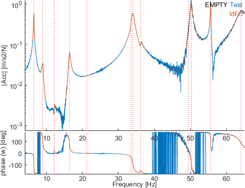
In the Ident tab, click on eopt to perform an broad band optimization (on the selected bandwidth so here on the full bandwidth) using the eopt strategy. Because many poles are present in the band, this algorithm is stuck in a local minimum and the result does not improve much the result.The figure below shows the transfer and the identification of the sensor 1001.03 (channel 2 in iiplot).
Run
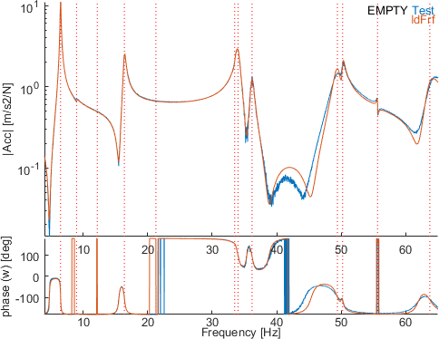
Click now on eup to use the other strategy, still on the whole bandwidth. The result deeply improves the identification quality : the same transfer is shown below after the optimization.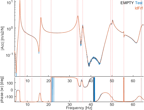
Nevertheless, some transfers still present a quite bad identification, like for instance sensors 2201.08 and 2301.07.
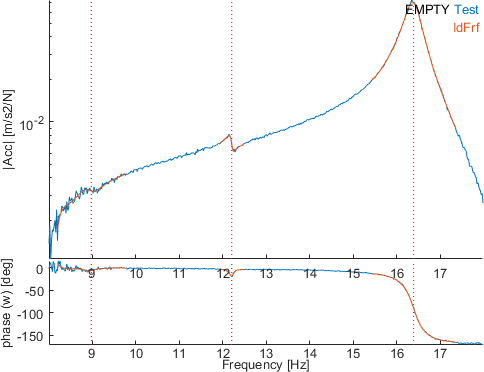
An interesting observation is that if a smaller band is selected where the fit is poor, without updating the poles, a new identification of the residues may lead to a better identification quality.
Run
Select a narrow band with the button wmo between 8 and 18 Hz. Click then on the button est to perform a new identification of the residues inside this band without updating the poles. Looking at the same channels as before (sensors 2201.08 and 2301.07), the fitting quality is clearly improved.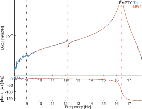
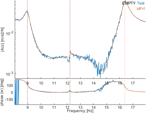
This is due to the fact that taking into account the poles outside this frequency band (especially the noisy first mode) leads to a bias of identification inside this band.
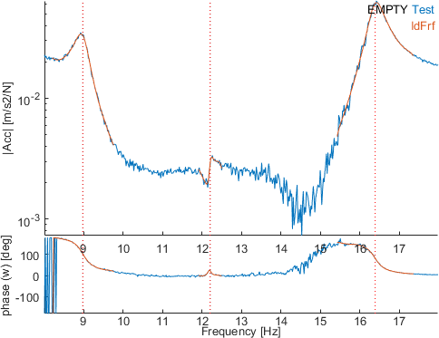
The difficulty is that it is not easy to define which frequency bands can be identified together. To deal with this issue, the sequential local identification of residuals estlocalpole can be used. Two version of this strategy have been developped to perform pole updating in addition to residue identification on narrow bands arround each mode : eoptSeq and eupSeq.
Run
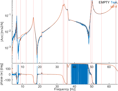
Click on eoptSeq to perform the sequential optimization. You can perform this optimization several times until convergence if needed.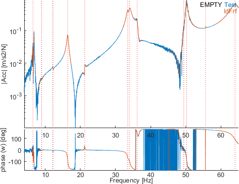
The vizualisation of the identification on the same band than previously shows a very good fit arround each mode.
Once a good complex residue model obtained, one often seeks models that verify other properties of minimality, reciprocity or represented in the second order mass, damping, stiffness form. These approximations are provided using the id_rm and id_nor algorithms as detailed in section 2.9.
The id_rc algorithm (see [19][18]) seeks a non linear least squares approximation of the measured data
| (2.7) |
for models in the nominal pole/residue form (also often called partial fraction expansion [20])
| (2.8) |
or its variants detailed under res .
These models are linear functions of the residues and residual terms [Rj,E,F] and non linear functions of the poles λj. The algorithm thus works in two stages with residues found as solution of a linear least-square problem and poles found through a non linear optimization.
The id_rc function (idcom eup command) uses an ad-hoc optimization where all poles are optimized simultaneously and steps and directions are found using gradient information. This algorithm is usually the most efficient when optimizing more than two poles simultaneously, but is not guaranteed to converge or even to improve the result.
The id_rcopt function (idcom eopt command) uses a gradient or conjugate gradient optimization. It is guaranteed to improve the result but tends to be very slow when optimizing poles that are not closely spaced (this is due to the fact that the optimization problem is non convex and poorly conditioned). The standard procedure for the use of these algorithms is described in section 2.2.3. Improved and more robust optimization strategies are still considered and will eventually find their way into the SDT.


