
 PDF Index
| SDT-base
Contents
Functions
PDF Index |
Correlation criteria seek to analyze the similarity and differences between two sets of results. Usual applications are the correlation of test and analysis results and the comparison of various analysis results.
Ideally, correlation criteria should quantify the ability of two models to make the same predictions. Since, the predictions of interest for a particular model can rarely be pinpointed precisely, one has to use general qualities and select, from a list of possible criterion, the ones that can be computed and do a good enough job for the intended purpose.
The ii_mac interface implements a number of correlation criteria. You should at least learn about the Modal Assurance Criterion (MAC) and Pseudo Orthogonality Checks (POC) (theoretical description can be found in ii_mac). These are very popular and should be used first. Other criteria should be used to get more insight when you don't have the desired answer or to make sure that your answer is really foolproof.
Again, there is no best choice for a correlation criterion unless you are very specific as to what you are trying to do with your model. Since that rarely happens, you should know the possibilities and stick to what is good enough for the job.
The following table gives a list of criteria implemented in the ii_mac interface.
| MAC | Modal Assurance Criterion (10.32). The most popular criterion for correlating vectors. Insensitive to vector scaling. Sensitive to sensor selection and level of response at each sensor. Main limitation : can give very misleading results without warning. Main advantage : can be used in all cases. A MAC criterion applied to frequency responses is called FRAC. |
| POC | Pseudo Orthogonality Checks (10.38). Required in some industries for model validation. This criterion is only defined for modes since other shapes do verify orthogonality conditions. Its scaled insensitive version (10.33) corresponds to a mass weighted MAC and is implemented as the MAC M commands. Main limitation: requires the definition of a mass associated with the known modeshape components. Main advantage : gives a much more reliable indication of correlation than the MAC. |
| Error | Modeshape pairing (based on the MAC or MAC-M) and relative frequency error and MAC correlation. |
| Rel | Relative error (10.39). Insensitive to scale when using the modal scale factor. Extremely accurate criterion but does not tell much when correlation poor. |
| COMAC | Coordinate Modal Assurance Criteria (three variants implemented in ii_mac) compare sets of vectors to analyze which sensors lead poor correlation. Main limitation : does not systematically give good indications. Main advantage : a very fast tool giving more insight into the reasons of poor correlation. |
| MACCO | What if analysis, where coordinates are sequentially eliminated from the MAC. Slower but more precise than COMAC. |
ii_mac describes the low-level calls to shape based correlation tools implemented in SDT, but to ease their practical usage, a dedicated MAC tab has been developed in the dock CoShape.
Here is a tutorial to present the classical GUI usage.
You will need the garteur example files, which can be found in SDTPath/sdtdemos/gart*.m. If these files are not present, click on the first step on the following tutorial in the HTML version of the documentation or download the patch at the address https://www.sdtools.com/contrib/garteur.zip and unzip the content in the folder SDTPath/sdtdemos.
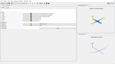
 Execute the command fecom('dockCoShape') to open an empty dock. You can also click on the button CoShape on the tree in SDT Root.
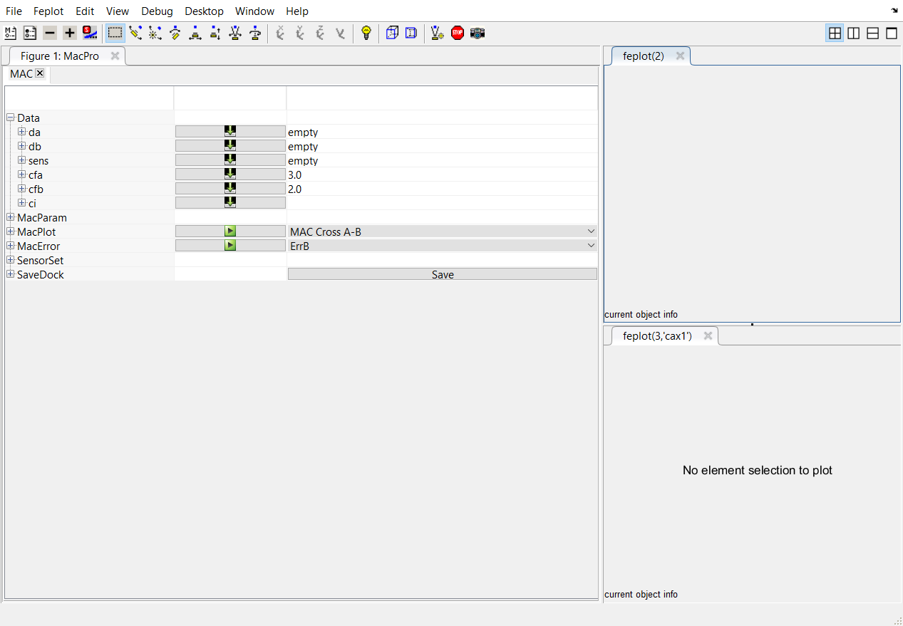
Click on  associated to the line sens to open the file containing the result of the superposition between a test wireframe and a FEM. This will open the import model window. Select the file to load : for this tutorial, the file is located at SDTPath/sdtdemos/gart_CoTopo.mat (it corresponds to the dock CoTopo saved file of the tutorial in section 3.1.1). Data is loaded and displayed in the two feplot figures. A brief description of the number of the observation is given in the table providing the number of sensors Nsens and the number of FEM DOFs NDof for the observation matrix.
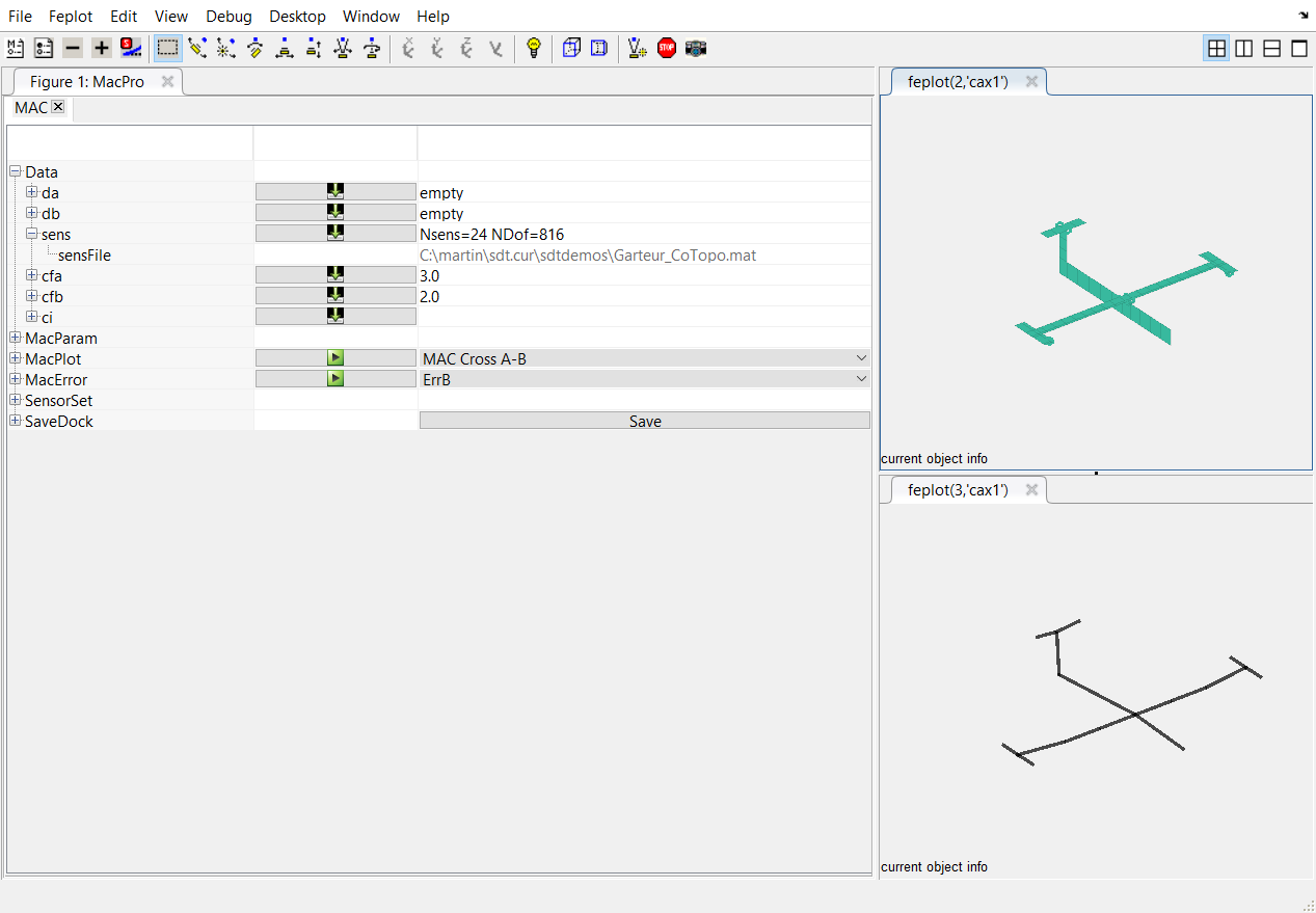
Click on associated to the line da to load the identified modes. In the opening window, select the file SDTPath/sdtdemos/gartid.unv. This will open the Unv tab in which you need to select the line containing the shape data and click on import.Do the same with the line db to load numerical modes. Select the file SDTPath/sdtdemos/gart_mdl.fil (mode computation result from abaqus).
The modeshapes are visible in both feplot figures.
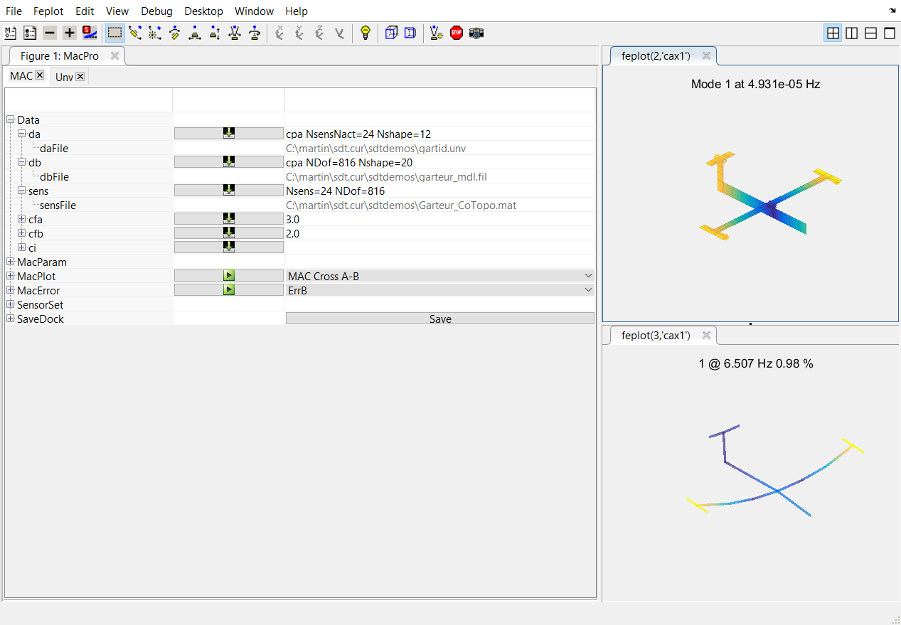
A brief description the data is displayed:
Click on associated to the line MacPlot to open the MAC matrix in a new window. 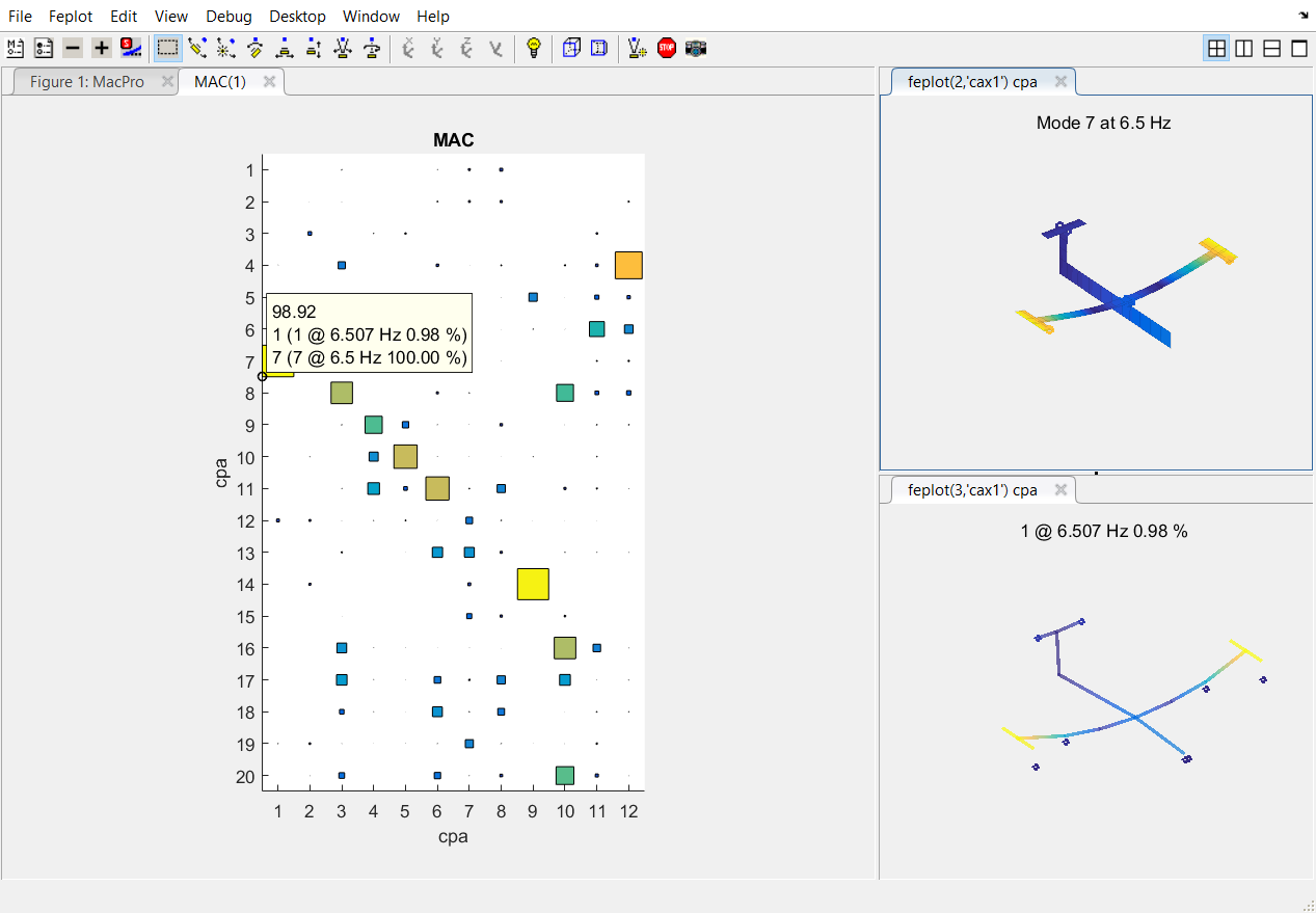
You can click on the square in the MAC matrix to interactively select the corresponding mode shapes in the feplot figure.
To pair more modes, expand the row MacError and allow a frequency shift Df of 20%. 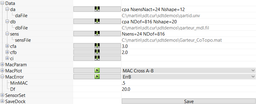
Click then on associated to the line MACError to open the MACError display in a new window.
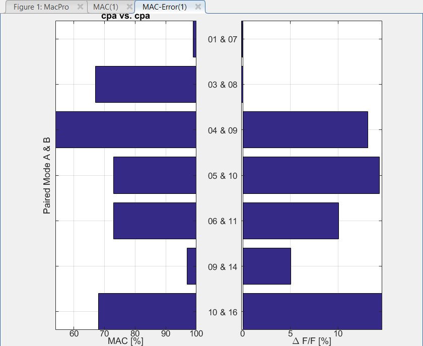
You can see here on the left the MAC value and on the right the relative frequency shift between the two sets of paired modes.
The criteria that make the most mechanical sense are derived from the equilibrium equations. For example, modes are defined by the eigenvalue problem (6.95). Thus the dynamic residual
| (3.1) |
should be close to zero. A similar residual (3.5) can be defined for FRFs.
The Euclidean norm of the dynamic residual has often been considered, but it tends to be a rather poor choice for models mixing translations and rotations or having very different levels of response in different parts of the structure.
To go to an energy based norm, the easiest is to build a displacement residual
| (3.2) |
and to use the strain  or kinetic
  energy norms for comparison.
Note that  need only be a reference stiffness that appropriately captures the system behavior. Thus for cases with rigid body modes, a pseudo-inverse of the stiffness (see section 6.2.4), or a mass shifted stiffness can be used. The displacement residual
  is sometimes called error in constitutive law (for reasons that have nothing to do with structural dynamics).
This approach is illustrated in the gartco demo and used for MDRE in fe_exp. While much more powerful than methods implemented in ii_mac, the development of standard energy based criteria is still a fairly open research topic.
Comparisons of frequency response functions are performed for both identification and finite element updating purposes.
The quadratic cost function associated with the Euclidean norm
| (3.3) |
is the most common comparison criterion. The main reason to use it is that it leads to linear least-squares problem for which there are numerically efficient solvers. (id_rc uses this cost function for this reason).
The quadratic cost corresponds to an additive description of the error on the transfer functions and, in the absence of weighting. It is mostly sensitive to errors in regions with high levels of response.
The log least-squares cost, defined by
| (3.4) |
uses a multiplicative description of the error and is as sensitive to resonances than to anti-resonances. While the use of a non-linear cost function results in much higher computational costs, this cost tends to be much better at distinguishing physically close dynamic systems than the quadratic cost (except when the difference is very small which is why the quadratic cost can be used in identification phases).
The utility function ii_cost computes these two costs for two sets of FRFs xf1 and xf2 (obtained through test and FE prediction using nor2xf for example). The evaluation of these costs provides a quick and efficient way to compare sets of MIMO FRF and is used in identification and model update algorithms.
Note that you might also consider the complex log of the transfer functions which would give a simple mechanism to take phase errors into account (this might become important for extremely accurate identification sometimes needed for control synthesis).
If the response at a given frequency can be expanded to the full finite element DOF set, you should consider an energy criterion based on the dynamic residual in displacement, which in this case takes the form
| (3.5) |
and can be used directly of test/analysis correlation and/or finite element updating.
Shape correlation tools provided by ii_mac can also be used to compare frequency responses. Thus the MAC applied to FRFs is sometimes called FRAC.


