Tutorial on handling orthotropic materials

SDT-visc Contents Functions

PDF Index

3.2 Tutorial on handling orthotropic materials

The first issue is to understand how material properties are stored in pl.html . xxx

Run

d_visco.tutomatortho.ddtransforms : sample manipulations

🧩code

%% step ddTransforms : sample manipulations
% keywords{var{mdl,pl},fcn{m_elastic,feutil}}

mdl=struct('Node',[],'Elt',[],...
    'pl',m_elastic('dbval1 Ortho1','dbval2 Steel'));

r1=feutil('getmat 1 -struct',mdl);
r2=m_elastic('FormulaOrtho',r1);%,struct('targ','ortho'))

% UD long fiber approximation
pl=m_elastic('formula{Em3.45e6, Ef380e6,Num.3, Nuf.33,rhom1.2e-6,rhof=1.95e-6,vf.6,unitMM,MatId10}');
feutil('_writepl MMSI',pl)
m_elastic('formula ortho',struct('pl',pl));

⚙️Keywords

name	cat	ToolTip	html
mdl	var	var.mdl	html
pl	var	pl	html
m_elastic	fcn	m_elastic	html
feutil	fcn	feutil	html

To ease transformations from other formats, m_elastic('FormulaLabToOrtho') supports transformations from tables to the SDT material format.

Run

d_visco.tutomatortho.lab2pl : Build from labels

🧩code

%% Step lab2pl : Build from labels 
% keywords{var{PrePl,pl},fcn{feform.eq.feform_feelas3d_4}}}

PrePl={'name','Type','E1','E2','E3','nu12','nu13','nu23','Gxy','G13','G23'
  'A',fe_mat('m_elastic','TM',6),126.810e3 8.908e3 8.908e3 .3 .3 .45 4.969e3 4.969e3 3.313e3};
PrePl(:,end+1)={'rho',1.6e-9};PrePl(:,end+1)={'MatId',1001};

mdl=feutil('setmat',mdl,struct('PrePl',{PrePl}));
%mdl=m_elastic('FormulaLabToOrtho',val,mdl);

% sdtweb fe_homo toortho

⚙️Keywords

name	cat	ToolTip	html
PrePl	var	var.PrePl	html
pl	var	pl	html
feform.eq.feform_feelas3d_4	fcn	eq.feform_feelas3d_4	html

Computation of fiber orientation has been the object of much work [47]. Draping commercial codes are available: QUICK-FORM, CATIA CPD, MSC Laminate Modeller, FiberSIM. SDT only seeks to allow incorporation of results of such software.

incorporating material orientations in element properties coordm requires definition of a property per element and is typically not compatible with variable orientation found when laying up plies.
element wise EltOrient stack entry is most relevant for thin plies since orientation changes at inter-ply boundaries. This is typically stored as a structure with .bas and .EltId fields. Usually the transform from material to global orientation TGL=reshape(bas(7:15),3,3). TensorT=feval(m_elastic(''),TGL) returns a structure with tensor transforms. Thus DDL=r4.tLG*DDG*r4.tGL corresponds to the coordinate transform.
d_visco('ScriptEltOrient') provides a sample script.
node wise NodeOrient stack entry can be used to model configurations with smooth property gradients.

d_visco.tutomatortho.loadmesh : show material orientation

🧩code

%% step loadMesh : show material orientation 
% keywords{var{MeshCfg,RunCfg},fcn{}}

li={'MeshCfg{d_mesh(blade),compA,}';
      'RunCfg{feplot}'};
RT=struct('nmap',vhandle.nmap);RT.nmap('CurExp')=li;
r2=sdtm.range.RT);mo2=r2.nmap('CurModel');%d2=mo2.nmap('CurTime');


fecom('colorfacew-alpha0')
fecom showmap EltOrient{d1{deflen,.3,edgecolor,r},d2{deflen,.3,edgecolor,g}}

mo3=feutil('orientNodeElt',mo2,struct('bas',[1 1 0  12 6  11]));
c20=feplot(20);c20.model=mo3; fecom('colorfacew-alpha0')
fecom showmap EltOrient{d1{deflen,.3,edgecolor,r},d2{deflen,.3,edgecolor,g}}
fecom(c20,';view4;viewv+180;views+90')

⚙️Keywords

name	cat	ToolTip
MeshCfg	var
RunCfg	var

d_visco.tutomatortho.ply_to_layer_homog : build layer volume law from plies

🧩code

%% Step ply_to_layer_homog : build layer volume law from plies

li={m_elastic('database{namePlyA,Matid10}','Ortho1');
    m_elastic('database{namePlyB,Matid11}','Ortho2');
  };li(:,3)={'mat'};li(:,2)=cellfun(@(x)x.name,li(:,1),'uni',0);
mo2=stack_set(mo2,li(:,[3 2 1]));

st1=(['formulaOrthoArea{AreaA1,MatId 1000,', ...
  'laminate 10 .05 90     11 .05 -45  11 .05 45  10  .05 90,' ...
  'silent0}']);
mo2=m_elastic(st1,mo2);mo2.Stack

% Area : zone with similar layup
% PlyNum : unique number of given ply. First Intrado ? 
% Theta : angle of ply
% Thick 
% PlyType : X/U 
% MatName : (points to matM) 
% CommentIndex 

%model.il=p_shell('dbval 101 laminate 3 1.3e-3 0', ...
% 'dbval 202 laminate 2 .25e-3 0 3 1.3e-3 0 2 .25e-3 0', ...
% 'dbval 302 laminate 2 .25e-3 0 3 1.3e-3 0 2 .25e-3 0');

⚙️Keywords

1
empty

d_visco.tutomatortho.orthosensib : sensitivity matrix

🧩code

%% Step OrthoSensib : sensitivity matrix
% d_visco('TutoMatOrtho -s{loadMesh}');
% update sdtweb comp12 TestbedScriptLocal
% comp13('SolveEFracNom'); % Energy Fraction table
% comp13('SolveESplit'); % Localize the energy fractions
% sdtweb _tag t_visco Comp25CutI

comp13('setSolve',struct('Omega',0,'MatId',1,'Split','ortho'))
PA=comp13('ParamVh');cf=feplot(mo2);
PA.mdl=stack_set(mo2,'info','EigOpt',[5 10 1e3]);
comp13('setProject',struct('name',mo2.name,'root',sprintf('BladeA')));
comp13('solveMVR'); % Reduce with components
comp13('setSolve',struct('IndMode','rb+(1:4)'))
comp13('solveEFracNom');  % comgui imwrite
comp13('solveESplit');fecom scc2e-3

if sdtweb('_TutoNeed','figgen')
 comgui('imwrite',1,'@tempdir/sdtdemos/plots/d_visco_TutoMatOrtho_EFracNom.png')
 fecom('ch1')
 comgui('imwrite',2,'@tempdir/sdtdemos/plots/d_visco_TutoMatOrtho_ESplit.png')
end

⚙️Keywords

1
empty

d_visco.tutomatortho.impmatrix : use of implicit matrices

🧩code

%% Step ImpMatrix : use of implicit matrices 

mo3=fe_caseg('ParMatCut',mo2,'groupall',struct('lab','Ortho','value',1));
mo3=fe_caseg('assemble -matdes -1 -SE',mo3);
if isa(mo3.K{1},'double');mo3.K(1)=[];mo3.Klab(1)=[];mo3.Opt(:,1)=[];end
c5=feplot(5);c5.model=mo3; c5.def=fe_eig(mo3,[5 20 1e3]);
c5.sel(1)='urn.EnerAtNode{sel{MatID1},KObs{2},os{CmParulaB,CbTR{String,eCL}}';



%% endTuto

⚙️Keywords

1
empty

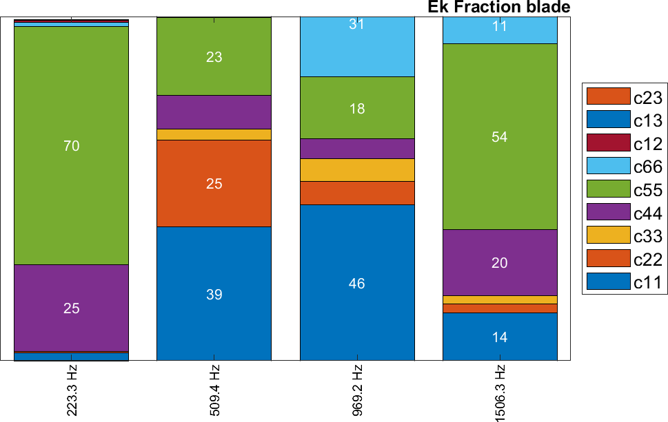
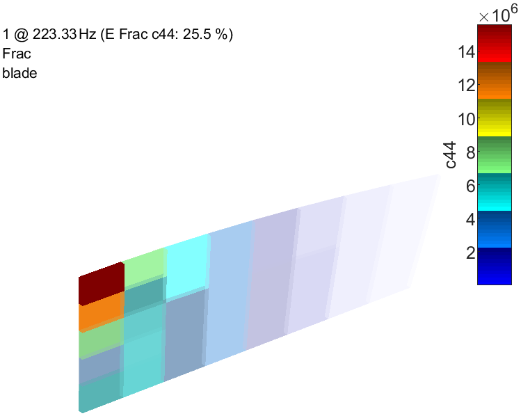
Run . It is often interesting to analyze how different components of an orthotropic constitutive law contribute to the strain energy. The two standard plots are

Figure 3.1: Left : EFracNom energy fraction per component. Right : distribution of energy