PDF Index
|
Contents
Functions
PDF Index |
Sensors are used for test/analysis correlation and in analysis for models where one wants to post-process partial information by using an observation equation {y}=[c]{q}. This general objective is supported by the use of SensDof entries. This section addresses the following issues
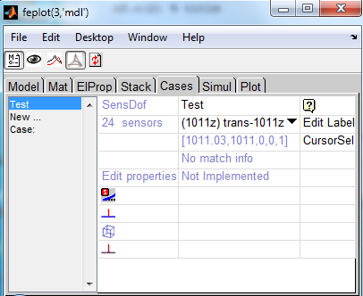
Using the feplot properties GUI, one can edit and visualize sensors. The following example loads ubeam model, defines some sensors and opens the sensor GUI.
model=demosdt('demo ubeam-pro');
cf=feplot; model=cf.mdl;

model=fe_case(model,'SensDof append trans','output',...
    [1,0.0,0.5,2.5,0.0,0.0,1.0]); %  add a translation sensor
model=fe_case(model,'SensDof append triax','output',8); % add triax sensor
model=fe_case(model,'SensDof append strain','output',...
    [4,0.0,0.5,2.5,0.0,0.0,1.0]); %  add strain sensor

model=fe_case(model,'sensmatch radius1','output'); % match sensor set 'output'

fecom(cf,'promodelviewon');
fecom(cf,'curtab Cases','output'); % open sensor GUI
Clicking on Edit Label one can edit the full list of sensor labels.
The whole sensor set can be visualized as arrows in the feplot figure clicking on the eye button on the top of the figure. Once visualization is activated one can activate the cursor on sensors by clicking on CursorSel. Then one can edit sensor properties by clicking on corresponding arrow in the feplot figure.
The icons in the GUI can be used to control the display of wire-frame, arrows and links.
Experimental setups can be defined with a cell array containing all the information relative to the sensors (only displacement/velocity/acceleration sensors are currently supported). This array is meant to be filled any table editor, possibly outside MATLAB. Using EXCEL you can read it with data=sdtacx('excel read filename',sheetnumber).
The first row gives column labels (the order in which they are given is free). Each of the following rows defines a sensor. Known column headers are
| 'dir x y z' | Direction of measurement specified trough its components in global coordinates (the vector is normalized). |
| 'X' | [1 0 0], in the reference frame |
| 'Y' | [0 1 0], in the reference frame |
| 'Z' | [0 0 1], in the reference frame |
| 'N' | normal to the element(s) to which the sensor is matched (automatically detected in the subsequent call to SensMatch) |
| 'TX' | tangent to matched surface in the N,X plane. |
| 'TY' | tangent to matched surface in the N,Y plane |
| 'TZ' | tangent to matched surface in the N,Z plane |
| 'N^TX' | tangent orthogonal to the N,X plane |
| 'N^TY' | tangent orthogonal to the N,Y plane |
| 'N^TZ' | tangent orthogonal to the N,Z plane |
| 'laser xs ys zs' | where (xs,ys,zs) are the coordinates of the primary or secondary source (when mirrors are used). |
| 'FEM 10.01' | associated FEM DOF |
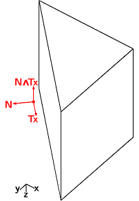
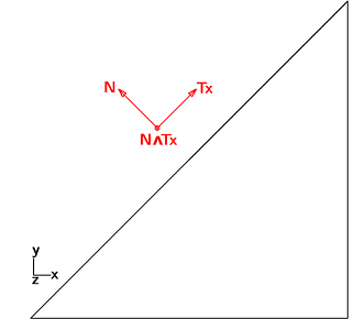
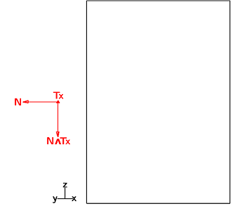
triax sensors are dealt with by defining three sensors with the same 'lab' but different 'SensId' and 'DirSpec'. In this case, a straightforward way to define the measurement directions is to make the first axis be the normal to the matching surface. The second axis is then forced to be parallel to the surface and oriented along a preferred reference axis, allowed by the possibility to define 'T*'. The third axis is therefore automatically built so that the three axes form a direct orthonormal basis with a specification such as N^T*. Note that there is no need to always consider the orthonormal basis as a whole and a single trans sensor with either 'T*' or N^T* as its direction of measure can be specified.
In the example below, one considers a pentahedron element and aims to observe the displacement just above the slanted face. The first vector is the normal to that face whose coordinates are [−√2/2,√2/2,0]. The second one is chosen (i.) parallel to the observed face, (ii.) in the (x,y) plane and (iii.) along x axis, so that its coordinates are [√2/2,√2/2,0]. Finally, the coordinates of the last vector can only be [0,0,−1] to comply with the orthonormality conditions. The resulting sensor placement is depicted in figure 4.11
cf=feplot;cf.model=femesh('testpenta6');fecom('triax');

% sensor definition as cell array
tcell={'lab', 'SensType','SensId','X','Y','Z','DirSpec';...
      'sensor 1','',      1.02,.4,.6,.5,'N';
      'sensor 2','',      1.01,.4,.6,.5,'TX';
      'sensor 3','',      2.01,.4,.6,1.,'dir 1 -1 1';
      'sensor 4','',      1.09,.4,.6,.5,'N^TX'
      'sensor 5','',      3.01,[],[],[],'FEM 5.01'
      'sensor 6','',      4.02, 1, 0, 1,'Y'
      };disp(tcell)
%sens=fe_sens('tdoftable',tcell);
cf.mdl=fe_case(cf.mdl,'SensDof','Test',tcell);
cf.mdl=fe_case(cf.mdl,'SensMatch radius1','Test','selface');
fecom(cf,'curtab Cases','Test'); fecom(cf,'ProViewOn')% open sensor GUI
sens=fe_case(cf.mdl,'sens');
fe_sens('tdoftable',cf,'Test') % see summary of match results
fname=fullfile(sdtdef('tempdir'),'SensSpec.xls');
if ~isunix % Test write to excel to illustrate ability to reread
 xlswrite(fname,tcell,'Sensors');
 sdtweb('_link',sprintf('open(''%s'')',fname))
end
It is now possible to generate the experimental setup of the ubeam example described in the previous section by the means of a single cell array containing the data relative to both the trans and triax sensors.
model=demosdt('demo ubeam-pro');
cf=feplot; model=cf.mdl;
n8=feutil('getnode NodeId 8',model); % triax pos.
tdof={'lab','SensType','SensId','X','Y','Z','DirSpec';...
      'sensor1 - trans','',1,0.0,0.5,2.5,'Z';
      'sensor2 - triax','',2,n8(:,5),n8(:,6),n8(:,7),'X';
      'sensor2 - triax','',3,n8(:,5),n8(:,6),n8(:,7),'Y';
      'sensor2 - triax','',4,n8(:,5),n8(:,6),n8(:,7),'Z'};
sens=fe_sens('tdoftable',tdof);
cf.mdl=fe_case(cf.mdl,'SensDof','output',sens);
cf.mdl=fe_case(cf.mdl,'SensMatch radius1');
fecom(cf,'curtab Cases','output'); % open sensor GUI
This is a reference section on SensDof case entries. A tutorial on the basic configuration with a test wire frame and translation sensors is given in section 2.7. SensDof entries can contain the following fields
| sens.Node | (optional) node matrix for sensor nodes that are not in the model. When defined, all node numbers in sens.tdof should refer to these nodes. The order typically differs from that in .tdof, you can get the positions with fe_sens('tdofNode',model,SensName). |
| sens.Elt | element description matrix for a wire-frame display of the sensors (typically for test wire-frames). |
| sens.bas | Coordinate system definitions for sens.Node, see fe_sens basis |
| sens.tdof | see details below. |
| sens.DOF | DOF definition vector for the analysis (finite element model). It defines the meaning of columns in sens.cta. |
| sens.cta | is an observation matrix associated with the observation equation {y}=[c]{q} (where q is defined on sens.DOF ). This is built using the fe_case sens command illustrated below. |
| sens.Stack | cell array with one row per sensor giving 'sens','SensorTag',data with data is a structure. SensorTag is obtained from SensId (first column of tdof) using feutil('stringdof',SensId). It is used to define the tag uniquely and may differ from the label that the user may want to associated with a sensor which is stored in data.lab. |
The sens.tdof field declares translation sensors and their directions
NodeId>0 corresponds is for use of model.Node locations and sens.Node should not be defined.
NodeId<0 is used to look for the node position in sens.Node rather than model.Node. Mixed definitions (some NodeId positive and other negative) are not supported.
Most initialization calls accept the specification of a physical x y z position, a .vert0 field is then defined.
All sensors are generated with the command
fe_case(model,'SensDof <append, combine> Sensor_type',Sensor,data,SensLab)
Sensor is the case entry name to which sensors will be added. data is a structure, a vector, or a matrix, which describes the sensor to be added. The nature of data depends on Sensor_type as detailed below. SensLab is an optional cell array used to define sensor labels. There should be as much elements in SensLab as sensors added. If there is only one string in the cell array SensLab, it is used to generate labels substituting for each sensor $id by its SensId, $type by its type (trans, strain ...), $j1 by its number in the set currently added. If SensLab is not given, default label generation is $type_$id.
In the default mode ('SensDof' command), new sensors replace any existing ones. In the append mode ('SensDof append'), if a sensor is added with an existing SensID, the SensID of new sensor will changed to a free SensID value. In the combine mode ('SensDof combine'), existing sensor with the same SensID will be replaced by the new one.
Relative displacement sensor or relative force sensor (spring load). Data passed to the command is [NodeID1 NodeID2].
This sensor measures the relative displacement between NodeID1 and NodeID2, along the direction defined from NodeID1 to NodeID2. One can use the command option -dof in order to measure along the defined DOF directions (mandatory if the two nodes are coincident). As many sensors as DOF are then added. For a relative force sensor, on can use the command option -coef to define the associated spring stiffness (sensor value is the product of the relative displacement and the stiffness of the spring).
If some DOF are missing, the sensor will be generated with a warning and a partial observation corresponding to the found DOF only.
The following example defines 3 relative displacement sensors (one in the direction of the two nodes, and two others along x and y):
model=demosdt('demo ubeam-pro')
data=[30 372];
model=fe_case(model,'SensDof append rel','output',data);
model=fe_case(model,'SensDof append rel -dof 1 2','output',data);
General sensors are defined by a linear observation equation. This is a low level definition that should be used for sensors that can't be described otherwise. Data passed to the command is a structure with field .cta (observation matrix), .DOF DOF associated to the observation matrix, and possibly .lab giving a label for each row of the observation matrix.
The following example defines a general sensor
model=demosdt('demo ubeam-pro');
Sensor=struct('cta',[1 -1;0 1],'DOF',[8.03; 9.03]);
model=fe_case(model,'SensDof append general','output',Sensor);
Translation sensors (see also section 2.7.2) can be specified by giving
[DOF]
[DOF, BasID]
[SensID, NodeID, nx, ny, nz]
[SensID, x, y, z, nx, ny, nz]
This is often used with wire frames, see section 2.7.2. The definition of test sensors is given in section 3.1.1.
The basic case is the measurement of a translation corresponding the main directions of a coordinate system. The DOF format (1.02 for 1y, see section 7.5) can then be simply used, the DOF values are used as is then used as SensID. Note that this form is also acceptable to define sensors for other DOFs (rotation, temperature, ...).
A number of software packages use local coordinate systems rather than a direction to define sensors. SDT provides compatibility as follows.
If model.bas contains local coordinate systems and deformations are given in the global frame (DID in column 3 of model.Node is zero), the directions nx ny nz (sens.tdof columns 3 to 5) must reflect local definitions. A call giving [DOF, BasID] defines the sensor direction in the main directions of basis BasID and the sensor direction is adjusted.
If FEM results are given in local coordinates, you should not specify a basis for the sensor definition, the directions nx ny nz (sens.tdof columns 3 to 5) should be [1 0 0], ... as obtained with a simple [DOF] argument in the sensor definition call.
When specifying a BasId, it the sensor direction nx ny nz is adjusted and given in global FEM coordinates. Observation should thus be made using FEM deformations in global coordinates (with a DID set to zero). If your FEM results are given in local coordinates, you should not specify a basis for the sensor definition. You can also perform the local to global transformation with
cGL= basis('trans E',model.bas,model.node,def.DOF)
def.def=cGL*def.def
The last two input forms specify location as x y z or NodeID, and direction nx ny nz (this vector need not be normalized, sensor value is the scalar product of the direction vector and the displacement vector).
One can add multiple sensors in a single call fe_case(model,'SensDof <append> trans', Name, Sensor) when rows of sensors contain sensor entries of the same form.
Following example defines a translation sensor using each of the forms
model=demosdt('demo ubeam-pro')
model.bas=basis('rotate',[],'r=30;n=[0 1 1]',100);
model=fe_case(model,'SensDof append trans','output',...
  [1,0.0,0.5,2.5,0.0,0.0,1.0]);
model=fe_case(model,'SensDof append trans','output',...
  [2,8,-1.0,0.0,0.0]);
model=fe_case(model,'SensDof append trans','output',...
  [314.03]);
model=fe_case(model,'SensDof append trans','output',...
  [324.03 100]);
cf=feplot;cf.sel(2)='-output';cf.o(1)={'sel2 ty 7','linewidth',2};
Sens.Stack entries for translation can use the following fields
| .vert0 | physical position in global coordinates. |
| .ID | NodeId for physical position. Positive if a model node, negative if SensDof entry node. |
| .match | cell array describing how the corresponding sensor is matched to the reference model. Columns are ElemF,elt,rstj,StickNode. |
One can simply define a set of sensors along model DOFs with a direct SensDof call model=fe_case(model,'SensDof','SensDofName',DofList). There is no need in that case to pass through SensMatch step in order to get observation matrix.
model=demosdt('demo ubeam-pro')
model=fe_case(model,'SensDof','output',[1.01;2.03;10.01]);
Sens=fe_case(model,'sens','output')
A triax is the same as defining 3 translation sensors, in each of the 3 translation DOF (0.01, 0.02 and 0.03) of a node. Use fe_case(model,'SensDof append triax', Name, NodeId) with a vector NodeId to add multiple triaxes. A positive NodeId refers to a FEM node, while a negative refers to a wire frame node.
For scanning laser vibrometer tests
fe_sens('laser px py pz',model,SightNodes,'SensDofName')
appends translation sensors based on line of sight direction from the laser scanner position px py pz to the measurement nodes SightNodes. Sighted nodes can be specified as a standard node matrix or using a node selection command such as 'NodeId>1000 & NodeId<1100' or also giving a vector of NodeId. If a test wire frame exists in the SensDofName entry, node selection command or NodeId list are defined in this model. If you want to flip the measurement direction, use a call of the form
cf.CStack{'output'}.tdof(:,3:5)=-cf.CStack{'output'}.tdof(:,3:5)
The following example defines some laser sensors, using a test wire frame:
cf=demosdt('demo gartfeplot'); model=cf.mdl;% load FEM
TEST=demosdt('demo garttewire');  % see sdtweb('pre#presen')
TEST.tdof=[];%Define test wire frame, but start with no tdof
model=fe_case(model,'SensDof','test',TEST)
model=fe_case(model,'SensDof Append Triax','test',-TEST.Node(1))

% Add sensors on TEST wire frame location
model=fe_sens('laser 0 0 6',model,-TEST.Node(2:end,1),'test');
% Show result
fecom('curtab Cases','output'); fecom('proviewon');
To add a sensor on FEM node you would use model=fe_sens('laser 0 0 6',model,20,'test'); but this is not possible here because SensDof entries do not support mixed definitions on test and FEM nodes.
Note that an extended version of this functionality is now discussed in section 4.7. Strain sensors can be specified by giving
[SensID, NodeID]
[SensID, x, y, z]
[SensID, NodeID, n1x, n1y, n1z]
[SensID, x, y, z, n1x, n1y, n1z]
[SensID, NodeID, n1x, n1y, n1z, n2x, n2y, n2z]
[SensID, x, y, z, n1x, n1y, n1z, n2x, n2y, n2z]
when no direction is specified 6 sensors are added for stress/strains in the x, y, z, yz, zx, and xy directions (SensId is incremented by steps of 1). With n1x n1y n1z (this vector need not be normalized) on measures the axial strain in this direction. For shear, one specifies a second direction n2x n2y n2z (this vector need not be normalized) (if not given n2 is taken equal to n1). The sensor value is given by {n2}T[є]{n1}.
Sensor can also be a matrix if all rows are of the same type. Then, one can add a set of sensors with a single call to the fe_case(model,'SensDof <append> strain', Name, Sensor) command.
Following example defines a strain sensor with each possible way:
model=demosdt('demo ubeam-pro')
model=fe_case(model,'SensDof append strain','output',...
  [4,0.0,0.5,2.5,0.0,0.0,1.0]);
model=fe_case(model,'SensDof append strain','output',...
  [6,134,0.5,0.5,0.5]);
model=fe_case(model,'SensDof append strain','output',...
  [5,0.0,0.4,1.25,1.0,0.0,0.0,0.0,0.0,1.0]);
model=fe_case(model,'SensDof append strain','output',...
  [7,370,0.0,0.0,1.0,0.0,1.0,0.0]);
Stress sensor.
It is the same as the strain sensor. The sensor value is given by {n2}T[σ]{n1}.
Following example defines a stress sensor with each possible way:
model=demosdt('demo ubeam-pro')
model=fe_case(model,'SensDof append stress','output',...
  [4,0.0,0.5,2.5,0.0,0.0,1.0]);
model=fe_case(model,'SensDof append stress','output',...
  [6,134,0.5,0.5,0.5]);
model=fe_case(model,'SensDof append stress','output',...
  [5,0.0,0.4,1.25,1.0,0.0,0.0,0.0,0.0,1.0]);
model=fe_case(model,'SensDof append stress','output',...
  [7,370,0.0,0.0,1.0,0.0,1.0,0.0]);
Element formulations (see section 6.1) include definitions of fields and their derivatives that are strain/stress in mechanical applications and similar quantities otherwise. The general formula is {є}=[B(r,s,t)]{q}. These (generalized) strain vectors are defined for all points of a volume and the default is to use an exact evaluation at the location of the sensor.
In practice, the generalized strains are more accurately predicted at integration points. Placing the sensor arbitrarily can generate some inaccuracy (for example stress and strains are discontinuous across element boundaries two nearby sensors might give different results). The -stick option can be used to for placement at specific gauss points. -stick by itself forces placement of the sensor and the center of the matching element. This will typically be a more appropriate location to evaluate stresses or strains.
To allow arbitrary positioning some level of reinterpolation is needed. The procedure is then to evaluate strain/stresses at Gauss points and use shape functions for reinterpolation. The process must however involve multiple elements to limit interelement discontinuities. This procedure is currently implemented through the fe_caseg('StressCut') command, as detailed in section 4.7.
Resultant sensors measure the resultant force on a given surface. Note that the observation of resultant fields is discussed in section 4.7.3. They can be specified by giving a structure with fields
| .ID | sensor ID. |
| .EltSel | FindElt command that gives the elements concerned by the resultant. |
| .SurfSel | FindNode command that gives the surface where the resultant is computed. |
| .dir | with 3 components direction of resultant measurement, with 6 origin and direction of resulting moment in global coordinates. This vector need not be normalized (scalar product). For non-mechanical DOF, .dir can be a scalar DOF ( .21 for electric field for example) |
| .type | contains the string 'resultant'. |
Following example defines a resultant sensor:
model=demosdt('demo ubeam-pro')
Sensor.ID=1;
Sensor.EltSel='WithNode{z==1.25} & WithNode{z>1.25}';
Sensor.SurfSel='z==1.25';
Sensor.dir=[0.0 0.0 1.0];
Sensor.type='resultant';
model=fe_case(model,'SensDof append resultant','output',Sensor);
Resultant sensors are not yet available for superelements model.
This command is used after SensMatch to build the observation equation that relates the response at sensors to the response a DOFs
| (4.1) |
where the c matrix in stored in the sens.cta field and DOFs expected for q are given in sens.tdof.
After the matching phase, one can build the observation matrix with
SensFull=fe_case(model,'sens',SensDofEntryName)
or when using a reduced superelement model
SensRed=fe_case(model,'sensSE',SensDofEntryName). Note that with superelements, you can also define a field .UseSE=1 in the sensor entry to force use of the reduced model. This is needed for the generation of reduced selections in feplot (typically cf.sel='-Test').
The following example illustrates nominal strategies to generate the observed shape, here for a static response.
model=demosdt('demoUbeamSens'); def=fe_simul('static',model);

% Manual observation, using {y} = [c] {q}
sens=fe_case(model,'sens');
def=feutilb('placeindof',sens.DOF,def); % If DOF numbering differs
% could use  sens=feutilb('placeindof',def.DOF,sens); if all DOF present
y=sens.cta*def.def
% Automated curve generation
C1=fe_case('sensObserve',model,'sensor 1',def)
Once sensors defined (see trans, ...), sensors must be matched to elements of the mesh. This is done using
model = fe_case(model,'sensmatch',SensDofEntryName);
You may omit to provide the name if there is only one sensor set. The command builds the observation matrix associated to each sensor of the entry Name, and stores it as a .cta field, and associated .DOF, in the sensor stack.
Storing information in the stack allows multiple partial matches before generating the global observation matrix. The observation matrix is then obtained using
Sens = fe_case(model,'sens',SensDofEntryName);
The matching operation requires finding the elements that contain each sensor and the position within the reference element shape so that shape functions can be used to interpolate the response. Typical variants are
model=fe_case(model,'sensmatch radius1.0',Name)
Note that this selection does not yet let you selected implicit elements within a superelement.
In an automated match, the sensor is not always matched to the correct elements on which the sensor is glued, you may want to ensure that the observation matrices created by these commands only use nodes associated to a subset of elements.
You can use a selection to define element subset on which perform the match. If you want to match one or more specific sensors to specific element subset, you can give cell array with SensId of sensor to match in a first column and with element string selector in a second column.
model=fe_case(model,'SensMatch',Name,{SensIdVector,'FindEltString'});
This is illustrated below in forcing the interpolation of test node 1206 to use FEM nodes in the plane where it is glued.
 cf=demosdt('demo gartte cor plot');
 fe_case(cf,'sensmatch -near')
 fecom('curtabCases','sensors');fecom('promodelviewon');
 % use fecom CursorSelOn to see how each sensor is matched.
 cf.CStack{'sensors'}.Stack{18,3}
 % modify link to 1206 to be on proper surface
 cf.mdl=fe_case(cf.mdl,'SensMatch-near',...
     'sensors',{1206.02,'withnode {z>.16}'});
 cf.CStack{'sensors'}.Stack{18,3}
 % force link to given node (may need to adjust distance)
 cf.mdl=fe_case(cf.mdl,'SensMatch-rigid radius .5','sensors',{1205.07,21});
 cf.CStack{'sensors'}.Stack{19,3}

 fecom('showlinks sensors');fecom('textnode',[1206 1205])
The generation of loads is less general than that of sensors. As a result it may be convenient to use reciprocity to define a load by generating the collocated sensor. When a sensor is defined, and the topology correlation performed with SensMatch, one can define an actuator from this sensor using
model=fe_case(model,'DofLoad SensDof',Input_Name,'Sens_Name:Sens_Nb') or for model using superelements
model=fe_case(model,'DofLoad SensDofSE',Input_Name,'Sens_Name:Sens_Nb').
Sens_Name is the name of the sensor set entry in the model stack of the translation sensor that defines the actuator, and Sens_Nb is its number in this stack entry. Thus Sensors:1 2 5 will define actuators with sensors 1, 2 and 5 for SensDof entry Sensors.
Input_Name is the name of the DofLoad entry that will be created in the model stack to describe the actuator.
Note that a verification of directions can be performed a posteriori using feutilb GeomRB.
This is discussed in section 2.7.3.
SDT 5.3 match strategies are still available. Only the arigid match has not been ported to SDT 6.1. This section thus documents SDT 5.3 match calls.
For topology correlation, the sensor configuration must be stored in the sens.tdof field and active FEM DOFs must be declared in sens.DOF. If you do not have your analysis modeshapes yet, you can use sens.DOF=feutil('getdof',sens.DOF). With these fields and a combined test/FEM model you can estimate test node motion from FEM results. Available interpolations are
At each point, you can see which interpolations you are using with
fe_sens('info',sens). Note that when defining test nodes in a local basis, the node selection commands are applied in the global coordinate system.
The interpolations are stored in the sens.cta field. With that information you can predict the response of the FEM model at test nodes. For example
 [model,def]=demosdt('demo gartte cor');
 model=fe_sens('rigid sensors',model); % link sensors to model
 % display sensor wire-frame and animate FEM modes
 cf=feplot; cf.model=model; cf.sel='-sensors';
 cf.def=def;fecom(';undefline;scd.5;ch7')